import numpy as np
import polars as pl

from funs import *
from plotnine import *
from polars import col as c
theme_set(theme_minimal())

from PIL import Image
import cv2
from ultralytics import YOLO

birds = pl.read_parquet("data/birds10.parquet")
birds_bbox = pl.read_csv("data/birds_1000.csv")
fsac = pl.read_csv("data/fsac.csv").select(c.filepath, c.photographer)20 Image Data
20.1 Setup
Load all of the modules and datasets needed for the chapter. In addition to the standard tools, we will use OpenCV (cv2) for image processing, PIL for image display, and the Ultralytics library for accessing pre-trained YOLO models.
20.2 Introduction
Images are among the most ubiquitous forms of data in the modern world. Every day, billions of photographs are captured on smartphones, satellites orbit the Earth generating terabytes of imagery, medical scanners produce detailed views of the human body, and security cameras record countless hours of video. The ability to extract meaningful information from these images has become one of the most important capabilities in data science.
At their core, digital images are simply arrays of numbers. Each pixel in an image stores numerical values representing color or intensity. Yet from these raw numbers emerge faces, objects, scenes, and stories. The challenge of image analysis lies in bridging this gap between low-level pixel values and high-level semantic meaning. How do we go from a grid of numbers to understanding that an image contains a bird, or that a person in a photograph is smiling, or that a tumor is present in a medical scan?
In this chapter, we explore several approaches to extracting information from images. We begin with basic properties that can be computed directly from pixel values, including brightness and color distributions. These simple features, while limited in their semantic power, provide useful descriptors for large collections of images and can reveal interesting patterns in visual datasets. We then turn to more sophisticated computer vision techniques that leverage deep learning models trained on millions of images. These models can detect objects, segment regions, and identify human poses with remarkable accuracy.
The progression in this chapter mirrors the broader evolution of computer vision as a field. Early approaches relied on hand-crafted features computed from pixel statistics. Modern methods use neural networks to learn relevant features directly from data. Both perspectives remain valuable: simple pixel-based features are interpretable, fast to compute, and often sufficient for exploratory analysis, while deep learning models offer unprecedented accuracy for complex recognition tasks. Understanding both approaches equips you to choose the right tool for each analytical situation.
Note that in addition to the task-specific models we explore here, images can also be converted into dense vector embeddings using the transfer learning techniques described in Chapter 15. These embeddings represent images as points in a high-dimensional space where visually or semantically similar images are close together. Once you have embeddings, all the familiar tools apply: you can train classifiers to predict categories, use dimensionality reduction techniques like PCA or UMAP to visualize collections, or apply clustering algorithms to discover groups of related images. The embedding approach is particularly powerful when you have domain-specific categories that don’t match the labels in pre-trained models.
20.3 Image Arrays
We will work with the birds image dataset, which contains photographs of ten species of birds. Each image has been preprocessed to a standard size and format, making it suitable for comparative analysis. The dataset includes species with distinctive coloration, from the brilliant yellow of canaries to the iridescent blues and greens of peacocks.
birds
shape: (1_555, 5)
| label | filepath | index | vit | siglip |
|---|---|---|---|---|
| str | str | str | list[f64] | list[f64] |
| "canary" | "media/birds10/00000.png" | "test" | [0.017947, -0.0305, … 0.003526] | [-0.00611, -0.042975, … -0.031687] |
| "canary" | "media/birds10/00001.png" | "train" | [0.024804, -0.045255, … -0.007233] | [-0.033767, -0.011978, … -0.020352] |
| "canary" | "media/birds10/00002.png" | "train" | [0.050587, -0.024486, … 0.029895] | [-0.033664, -0.008117, … -0.01725] |
| "canary" | "media/birds10/00003.png" | "train" | [0.047036, -0.038993, … -0.008446] | [-0.010029, -0.018192, … -0.009869] |
| "canary" | "media/birds10/00004.png" | "train" | [0.036349, -0.02734, … -0.018185] | [-0.027327, 0.003568, … -0.033407] |
| … | … | … | … | … |
| "swallow" | "media/birds10/01550.png" | "train" | [-0.022461, -0.025098, … -0.061945] | [-0.022029, -0.008476, … -0.003879] |
| "swallow" | "media/birds10/01551.png" | "train" | [-0.000212, -0.003448, … -0.058042] | [-0.02476, -0.016369, … 0.003875] |
| "swallow" | "media/birds10/01552.png" | "train" | [-0.012531, -0.006788, … -0.047077] | [-0.022153, 0.00765, … -0.011152] |
| "swallow" | "media/birds10/01553.png" | "test" | [-0.007587, -0.053535, … -0.046395] | [-0.005022, 0.00878, … -0.017564] |
| "swallow" | "media/birds10/01554.png" | "train" | [-0.01325, -0.032453, … -0.050751] | [-0.015117, -0.00685, … -0.029756] |
The dataset contains a filepath column pointing to each image file and a label column identifying the species. This structure, with metadata in a table and actual image files stored separately, is a common pattern for working with image datasets. It allows us to use familiar tabular data tools for filtering, grouping, and summarizing while keeping the image files in their native format.
To work with an image programmatically, we need to read it into Python as a numerical array. The OpenCV library provides the imread function for this purpose. Let’s load the first image in our dataset.
img = cv2.imread(birds.select(pl.col("filepath").get(0)).item())
img
array([[[ 18, 20, 21],
[ 22, 24, 25],
[ 23, 25, 26],
...,
[ 48, 48, 54],
[ 48, 47, 56],
[ 47, 46, 55]],
[[ 18, 20, 21],
[ 20, 22, 23],
[ 20, 22, 23],
...,
[ 50, 50, 56],
[ 49, 48, 57],
[ 47, 46, 55]],
[[ 12, 15, 19],
[ 11, 14, 18],
[ 12, 15, 19],
...,
[ 55, 53, 59],
[ 53, 51, 57],
[ 52, 50, 56]],
...,
[[133, 148, 180],
[147, 159, 187],
[126, 130, 149],
...,
[122, 98, 92],
[104, 81, 79],
[ 87, 66, 65]],
[[116, 133, 166],
[138, 152, 181],
[133, 140, 165],
...,
[113, 91, 86],
[106, 87, 90],
[ 87, 70, 74]],
[[ 89, 108, 141],
[127, 142, 174],
[140, 149, 176],
...,
[103, 82, 80],
[ 91, 74, 78],
[122, 107, 115]]], shape=(224, 224, 3), dtype=uint8)What we see is a NumPy array filled with numbers. Each number represents the intensity of a color channel at a specific pixel location. The values range from 0 (no intensity) to 255 (maximum intensity), using 8 bits per channel, which is the standard format for most digital images.
The shape of this array reveals the structure of the image data.
img.shape(224, 224, 3)The three dimensions correspond to height (number of rows of pixels), width (number of columns), and color channels. Most color images use three channels: red, green, and blue (RGB). However, OpenCV reads images in BGR order (blue, green, red), a historical convention from early computer vision libraries. This ordering rarely matters for analysis but becomes important when displaying images or converting between color spaces.
We can examine a small region of the array to see the actual pixel values. Here are the values for a 4×4 block of pixels in the upper-left corner.
img[:4, :4, :]array([[[18, 20, 21],
[22, 24, 25],
[23, 25, 26],
[22, 24, 25]],
[[18, 20, 21],
[20, 22, 23],
[20, 22, 23],
[19, 21, 22]],
[[12, 15, 19],
[11, 14, 18],
[12, 15, 19],
[15, 18, 22]],
[[17, 20, 24],
[13, 16, 20],
[13, 16, 20],
[14, 17, 21]]], dtype=uint8)Each pixel is represented by three values, one for each color channel. A pixel with values [255, 255, 255] would be pure white, while [0, 0, 0] would be pure black. Values like [255, 0, 0] represent pure blue (remember, OpenCV uses BGR ordering), [0, 255, 0] is green, and [0, 0, 255] is red.
One of the simplest statistics we can compute from an image is the mean of all pixel values.
img.mean()np.float64(119.86716757015306)This single number summarizes the overall intensity of the image. Higher values indicate brighter images (more pixels closer to 255), while lower values indicate darker images (more pixels closer to 0). While crude, this measure provides a starting point for understanding the visual characteristics of image collections.
20.4 Brightness
Let’s compute the mean brightness for every image in our bird dataset. This requires iterating through all images, loading each one, and computing its mean pixel value. We store the results and add them as a new column to our DataFrame.
results = []

for row in birds.iter_rows(named=True):
    img = cv2.imread(row["filepath"])
    results.append(img.mean())

birds = birds.with_columns(brightness = pl.Series(results))
birds
shape: (1_555, 6)
| label | filepath | index | vit | siglip | brightness |
|---|---|---|---|---|---|
| str | str | str | list[f64] | list[f64] | f64 |
| "canary" | "media/birds10/00000.png" | "test" | [0.017947, -0.0305, … 0.003526] | [-0.00611, -0.042975, … -0.031687] | 119.867168 |
| "canary" | "media/birds10/00001.png" | "train" | [0.024804, -0.045255, … -0.007233] | [-0.033767, -0.011978, … -0.020352] | 135.112989 |
| "canary" | "media/birds10/00002.png" | "train" | [0.050587, -0.024486, … 0.029895] | [-0.033664, -0.008117, … -0.01725] | 97.398424 |
| "canary" | "media/birds10/00003.png" | "train" | [0.047036, -0.038993, … -0.008446] | [-0.010029, -0.018192, … -0.009869] | 97.469866 |
| "canary" | "media/birds10/00004.png" | "train" | [0.036349, -0.02734, … -0.018185] | [-0.027327, 0.003568, … -0.033407] | 144.174758 |
| … | … | … | … | … | … |
| "swallow" | "media/birds10/01550.png" | "train" | [-0.022461, -0.025098, … -0.061945] | [-0.022029, -0.008476, … -0.003879] | 119.851436 |
| "swallow" | "media/birds10/01551.png" | "train" | [-0.000212, -0.003448, … -0.058042] | [-0.02476, -0.016369, … 0.003875] | 151.026155 |
| "swallow" | "media/birds10/01552.png" | "train" | [-0.012531, -0.006788, … -0.047077] | [-0.022153, 0.00765, … -0.011152] | 156.078922 |
| "swallow" | "media/birds10/01553.png" | "test" | [-0.007587, -0.053535, … -0.046395] | [-0.005022, 0.00878, … -0.017564] | 118.326265 |
| "swallow" | "media/birds10/01554.png" | "train" | [-0.01325, -0.032453, … -0.050751] | [-0.015117, -0.00685, … -0.029756] | 156.02357 |
Now we have a brightness value for each image. What can this simple statistic tell us about our photographs? Let’s examine the darkest images in the collection.
(
    birds
    .sort(c.brightness)
    .head(12)
    .pipe(DSImage.plot_image_grid, ncol=4)
)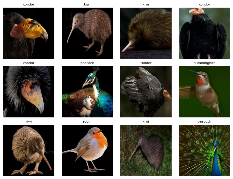
We see that the darkest images tend to have black backgrounds. This makes sense: a large area of pure black pixels (value 0) dramatically reduces the mean. The birds themselves may be brightly colored, but the dark backgrounds dominate the overall brightness calculation.
The brightest images show the opposite pattern.
(
    birds
    .sort(c.brightness, descending=True)
    .head(12)
    .pipe(DSImage.plot_image_grid, ncol=4)
)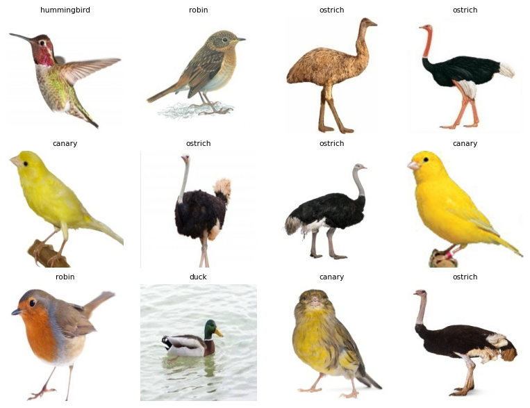
These images feature white or light-colored backgrounds, which push the mean toward higher values. This observation reveals an important limitation of simple pixel statistics: they capture properties of the entire image, including background, lighting conditions, and photographic style, not just the subject we care about. A dark bird photographed against a white background will have a higher brightness score than the same bird against a dark background.
Despite this limitation, brightness can reveal interesting patterns across categories. Here are the distributions of brightness by species.
(
    birds
    .pipe(ggplot, aes("reorder(label, brightness)", "brightness"))
    + geom_boxplot()
)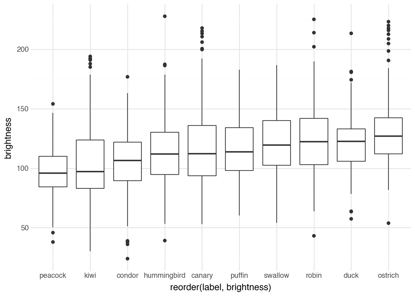
Ostriches have brighter images on average, followed by ducks and robins. Peacock images are the darkest. Why might this be? Consider how each species is typically photographed. Ostriches are often captured outdoors in bright savanna settings, while peacocks with their dark iridescent plumage are sometimes photographed against dramatic dark backgrounds that emphasize their colorful displays. The brightness distribution reflects not just the birds themselves but the entire photographic context.
20.5 Hue, Saturation, and Value
While brightness provides a single summary statistic, the RGB color model used by digital images is not ideal for describing color as humans perceive it. The HSV (Hue, Saturation, Value) color model offers a more intuitive representation that separates color information into three distinct components.
Hue represents the pure color itself, independent of how light or vivid it appears. Hue is measured as an angle around a color wheel, typically ranging from 0° to 360°. Red appears at 0° (and wraps around to 360°), yellow at 60°, green at 120°, cyan at 180°, blue at 240°, and magenta at 300°. This circular representation explains why red and magenta appear adjacent: they are neighbors on the color wheel.
Saturation measures the purity or intensity of a color. A fully saturated color contains no gray: it is vivid and intense. As saturation decreases, the color becomes more washed out, eventually becoming a pure gray at zero saturation. Saturation ranges from 0 (completely desaturated, gray) to 1 (fully saturated, pure color).
Value (also called brightness or lightness in related color models) indicates how light or dark the color is. A value of 0 produces black regardless of hue or saturation, while a value of 1 produces the brightest possible version of that hue and saturation combination.
The mathematical conversion from RGB to HSV proceeds as follows. Given RGB values normalized to the range [0, 1], we first compute:
\[ \begin{aligned} M &= \max(R, G, B) \\ m &= \min(R, G, B) \\ C &= M - m \end{aligned} \]
The value \(M\) is the maximum of the three channels, \(m\) is the minimum, and \(C\) (chroma) measures the range. The HSV components are then calculated as:
\[ V = M \]
\[ S = \begin{cases} 0 & \text{if } V = 0 \\ \frac{C}{V} & \text{otherwise} \end{cases} \]
\[ H = \begin{cases} 0° & \text{if } C = 0 \\ 60° \times \frac{G - B}{C} \mod 360° & \text{if } M = R \\ 60° \times \left(\frac{B - R}{C} + 2\right) & \text{if } M = G \\ 60° \times \left(\frac{R - G}{C} + 4\right) & \text{if } M = B \end{cases} \]
The value component is simply the maximum RGB value. Saturation measures how much the color differs from gray by comparing the range of RGB values to the maximum. Hue is computed by determining which RGB component is dominant and calculating the position around the color wheel.
OpenCV provides built-in functions for color space conversion. Here is how to convert an image from BGR to HSV.
img = cv2.imread(birds.select(pl.col("filepath").get(0)).item())

img_hsv = cv2.cvtColor(img, cv2.COLOR_BGR2HSV)
img_hsv.shape
(224, 224, 3)The resulting array has the same shape as the original, but now the three channels represent hue, saturation, and value instead of blue, green, and red. Note that OpenCV scales hue to the range [0, 179] (to fit in an 8-bit value while covering the full 360° range) and saturation and value to [0, 255].
20.6 Colors
With images represented in HSV color space, we can classify pixels by their dominant color. The hue value tells us where each pixel falls on the color wheel, allowing us to count how many pixels are predominantly red, orange, yellow, green, and so on.
Our helper method DSImage.compute_colors takes an HSV image and returns a dictionary with the proportion of pixels falling into each color category. It bins the hue values into segments corresponding to common color names and also accounts for the saturation and value (very dark or desaturated pixels are classified separately as black, white, or gray).
DSImage.compute_colors(img_hsv){'red': np.float64(6.048708545918367),
'orange': np.float64(8.326690051020408),
'yellow': np.float64(9.394929846938775),
'green': np.float64(0.06377551020408163),
'cyan': np.float64(0.005978954081632653),
'blue': np.float64(1.0981345663265305),
'purple': np.float64(0.007971938775510204),
'magenta': np.float64(0.04185267857142857),
'neutral': np.float64(75.01195790816327)}The output shows what fraction of pixels in this image fall into each color category. The proportions sum to 1, giving us a complete description of the color distribution.
We will cycle through the entire DataFrame and compute these color proportions for all images.
results = []

for row in birds.iter_rows(named=True):
    img = cv2.imread(row["filepath"])
    img_hsv = cv2.cvtColor(img, cv2.COLOR_BGR2HSV)
    results.append(DSImage.compute_colors(img_hsv))


results = pl.DataFrame(results)
birds = pl.concat([birds, results], how="horizontal")
birds
shape: (1_555, 15)
| label | filepath | index | vit | siglip | brightness | red | orange | yellow | green | cyan | blue | purple | magenta | neutral |
|---|---|---|---|---|---|---|---|---|---|---|---|---|---|---|
| str | str | str | list[f64] | list[f64] | f64 | f64 | f64 | f64 | f64 | f64 | f64 | f64 | f64 | f64 |
| "canary" | "media/birds10/00000.png" | "test" | [0.017947, -0.0305, … 0.003526] | [-0.00611, -0.042975, … -0.031687] | 119.867168 | 6.048709 | 8.32669 | 9.39493 | 0.063776 | 0.005979 | 1.098135 | 0.007972 | 0.041853 | 75.011958 |
| "canary" | "media/birds10/00001.png" | "train" | [0.024804, -0.045255, … -0.007233] | [-0.033767, -0.011978, … -0.020352] | 135.112989 | 8.968431 | 23.794244 | 6.806043 | 1.7578125 | 1.480788 | 0.0 | 0.0 | 0.0 | 57.192682 |
| "canary" | "media/birds10/00002.png" | "train" | [0.050587, -0.024486, … 0.029895] | [-0.033664, -0.008117, … -0.01725] | 97.398424 | 0.01993 | 30.29536 | 52.800143 | 0.049825 | 0.009965 | 0.932717 | 0.0 | 0.0 | 15.89206 |
| "canary" | "media/birds10/00003.png" | "train" | [0.047036, -0.038993, … -0.008446] | [-0.010029, -0.018192, … -0.009869] | 97.469866 | 0.0 | 26.546556 | 64.339525 | 0.007972 | 0.0 | 0.0 | 0.0 | 0.0 | 9.105947 |
| "canary" | "media/birds10/00004.png" | "train" | [0.036349, -0.02734, … -0.018185] | [-0.027327, 0.003568, … -0.033407] | 144.174758 | 0.288983 | 96.593989 | 0.454401 | 0.0 | 0.0 | 0.0 | 0.0 | 0.0 | 2.662628 |
| … | … | … | … | … | … | … | … | … | … | … | … | … | … | … |
| "swallow" | "media/birds10/01550.png" | "train" | [-0.022461, -0.025098, … -0.061945] | [-0.022029, -0.008476, … -0.003879] | 119.851436 | 0.061783 | 14.807876 | 0.655692 | 0.063776 | 0.121572 | 57.553412 | 0.0 | 0.0 | 26.73589 |
| "swallow" | "media/birds10/01551.png" | "train" | [-0.000212, -0.003448, … -0.058042] | [-0.02476, -0.016369, … 0.003875] | 151.026155 | 0.691566 | 2.451371 | 24.447943 | 0.089684 | 0.187341 | 3.386081 | 0.0 | 0.027902 | 68.718112 |
| "swallow" | "media/birds10/01552.png" | "train" | [-0.012531, -0.006788, … -0.047077] | [-0.022153, 0.00765, … -0.011152] | 156.078922 | 0.185348 | 11.820392 | 5.369101 | 0.053811 | 0.159439 | 64.845743 | 0.0 | 0.0 | 17.566167 |
| "swallow" | "media/birds10/01553.png" | "test" | [-0.007587, -0.053535, … -0.046395] | [-0.005022, 0.00878, … -0.017564] | 118.326265 | 0.007972 | 0.239158 | 0.159439 | 0.819117 | 0.185348 | 5.624203 | 0.0 | 0.0 | 92.964764 |
| "swallow" | "media/birds10/01554.png" | "train" | [-0.01325, -0.032453, … -0.050751] | [-0.015117, -0.00685, … -0.029756] | 156.02357 | 1.052296 | 20.938297 | 0.187341 | 0.155453 | 0.075733 | 0.277025 | 0.0 | 0.001993 | 77.311862 |
Now our dataset includes columns for each color category, enabling systematic analysis of color distributions across species. Let’s examine which images contain the most yellow.
(
    birds
    .sort(c.yellow, descending=True)
    .head(12)
    .pipe(DSImage.plot_image_grid, ncol=4)
)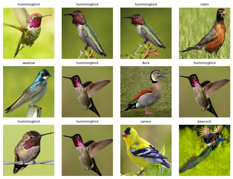
The images with the highest yellow proportions include many hummingbirds photographed near yellow-green foliage, as well as the expected yellow birds. This demonstrates how color analysis captures not just the subject but the entire scene.
We can compare the yellow content across species systematically.
(
    birds
    .pipe(ggplot, aes("reorder(label, yellow)", "yellow"))
    + geom_boxplot()
)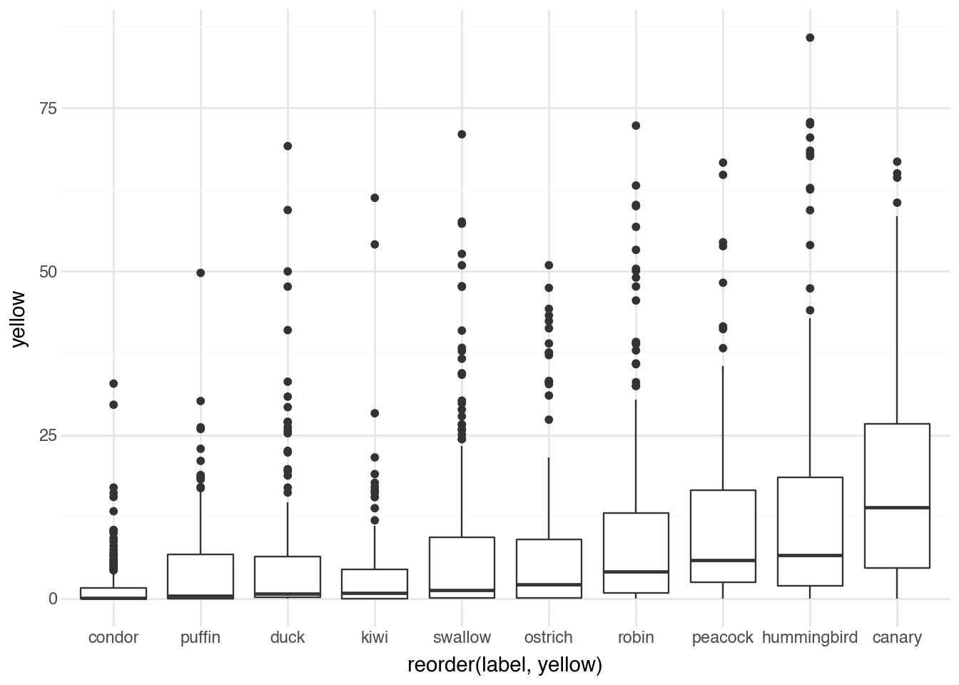
Canaries, as expected, have the highest yellow content on average. Their bright yellow plumage dominates the images. Other species show less yellow, with the distribution reflecting both the birds’ coloration and their typical photographic environments.
Peacocks, known for their brilliant blue-green displays, should show high values in the cyan range.
(
    birds
    .pipe(ggplot, aes("reorder(label, cyan)", "cyan"))
    + geom_boxplot()
)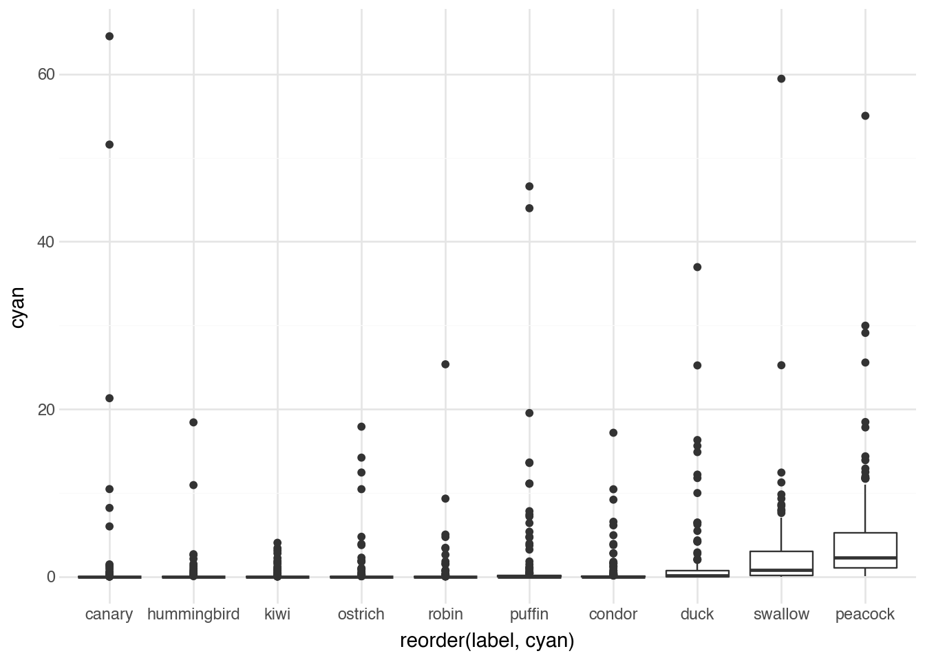
Indeed, peacocks lead in cyan content, reflecting their characteristic iridescent feathers that shimmer between blue and green. Parrots also show substantial cyan, while species like robins and canaries have minimal cyan in their typical coloration.
These color features, while simple to compute, provide useful descriptors for organizing and exploring image collections. They can identify outliers (an unusually red canary might indicate a different subspecies or unusual lighting), reveal patterns across categories, and serve as features for downstream machine learning tasks.
20.7 Object Detection
In Chapter 15 we saw how to use pre-trained deep learning models for image-level predictions, classifying entire images into categories. Object detection extends this capability by identifying and locating multiple objects within a single image. Rather than asking “what is in this image?”, object detection asks “what objects are in this image, and where are they?”
Modern object detection models output a set of bounding boxes, each consisting of four coordinates that define a rectangle enclosing a detected object, along with a class label and a confidence score. The model might report: “there is a person at coordinates (100, 50) to (200, 300) with 95% confidence, and a dog at (250, 100) to (350, 250) with 87% confidence.”
The YOLO (You Only Look Once) family of models represents the state of the art in real-time object detection. These models process entire images in a single forward pass through the network, making them remarkably fast while maintaining high accuracy. The architecture divides the image into a grid, with each cell responsible for predicting objects centered in that cell. This design enables the model to reason globally about the image while making localized predictions.
Training an object detection model requires labeled data where humans have drawn bounding boxes around objects and assigned class labels. The loss function combines several components:
\[ \mathcal{L} = \lambda_{\text{coord}} \mathcal{L}_{\text{box}} + \lambda_{\text{obj}} \mathcal{L}_{\text{obj}} + \lambda_{\text{cls}} \mathcal{L}_{\text{cls}} \]
The box loss \(\mathcal{L}_{\text{box}}\) penalizes errors in the predicted bounding box coordinates. Modern implementations often use Complete Intersection over Union (CIoU) loss, which considers the overlap between predicted and ground-truth boxes along with the distance between their centers and aspect ratio consistency:
\[ \mathcal{L}_{\text{CIoU}} = 1 - \text{IoU} + \frac{\rho^2(b, b^{gt})}{c^2} + \alpha v \]
where IoU is the intersection over union of the boxes, \(\rho(b, b^{gt})\) is the Euclidean distance between box centers, \(c\) is the diagonal length of the smallest enclosing box, and \(v\) measures aspect ratio consistency.
The objectness loss \(\mathcal{L}_{\text{obj}}\) trains the model to predict whether each grid cell contains an object. The classification loss \(\mathcal{L}_{\text{cls}}\) trains the model to correctly identify the class of detected objects. The \(\lambda\) coefficients balance these components during training.
Let’s load a pre-trained YOLO model and apply it to historical photographs.
model = YOLO("yolo11n.pt")For this analysis, we will use a collection of color photographs from the FSA-OWI (Farm Security Administration - Office of War Information) project, a remarkable documentary photography initiative from the 1930s and 1940s. These images captured American life during the Great Depression and World War II.
fsac
shape: (500, 2)
| filepath | photographer |
|---|---|
| str | str |
| "media/fsac/1a35266v.jpg" | "Alfred T. Palmer" |
| "media/fsac/1a34940v.jpg" | "Howard R. Hollem" |
| "media/fsac/1a34143v.jpg" | "Russell Lee" |
| "media/fsac/1a35375v.jpg" | "Alfred T. Palmer" |
| "media/fsac/1a34758v.jpg" | "Jack Delano" |
| … | … |
| "media/fsac/1a34359v.jpg" | "Marion Post Wolcott" |
| "media/fsac/1a34893v.jpg" | "Howard R. Hollem" |
| "media/fsac/1a34100v.jpg" | "Russell Lee" |
| "media/fsac/1a35045v.jpg" | "Howard Liberman" |
| "media/fsac/1a34863v.jpg" | "Howard R. Hollem" |
Here is an example of running object detection on one of these historical photographs.
pred = model.predict("media/fsac/1a35210v.jpg")
image 1/1 /Users/admin/gh/fds-py/media/fsac/1a35210v.jpg: 544x640 3 persons, 25.2ms
Speed: 1.0ms preprocess, 25.2ms inference, 0.8ms postprocess per image at shape (1, 3, 544, 640)
The model returns predictions that include bounding boxes, class labels, and confidence scores. We can visualize the detections by overlaying them on the original image.
rgb = cv2.cvtColor(pred[0].plot(), cv2.COLOR_BGR2RGB)
pil_img = Image.fromarray(rgb)
pil_img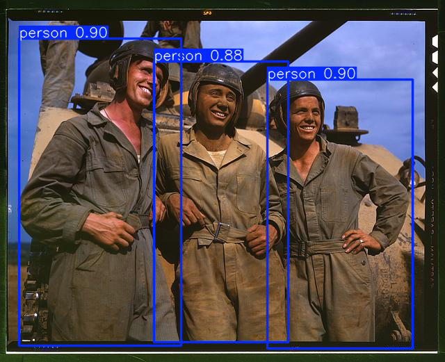
The visualization shows bounding boxes around detected objects, each labeled with the predicted class and confidence score. The model has been trained on the COCO dataset, which includes 80 common object categories such as person, car, dog, chair, and bicycle.
Let’s systematically count the number of people detected in each image across our collection.
results = []

for row in fsac.iter_rows(named=True):
    preds = model.predict(row["filepath"], verbose=False)[0]

    if preds.boxes is None:
        results.append(0)
        continue

    cls_ids = preds.boxes.cls.tolist()
    names = preds.names
    results.append(sum(names[int(c)] == "person" for c in cls_ids))


fsac = fsac.with_columns(people = pl.Series(results))
fsac
shape: (500, 3)
| filepath | photographer | people |
|---|---|---|
| str | str | i64 |
| "media/fsac/1a35266v.jpg" | "Alfred T. Palmer" | 0 |
| "media/fsac/1a34940v.jpg" | "Howard R. Hollem" | 0 |
| "media/fsac/1a34143v.jpg" | "Russell Lee" | 10 |
| "media/fsac/1a35375v.jpg" | "Alfred T. Palmer" | 1 |
| "media/fsac/1a34758v.jpg" | "Jack Delano" | 0 |
| … | … | … |
| "media/fsac/1a34359v.jpg" | "Marion Post Wolcott" | 8 |
| "media/fsac/1a34893v.jpg" | "Howard R. Hollem" | 1 |
| "media/fsac/1a34100v.jpg" | "Russell Lee" | 1 |
| "media/fsac/1a35045v.jpg" | "Howard Liberman" | 0 |
| "media/fsac/1a34863v.jpg" | "Howard R. Hollem" | 0 |
We can examine the images with the most detected people.
(
    fsac
    .sort(c.people, descending=True)
    .head(8)
    .pipe(DSImage.plot_image_grid, ncol=4, label_name="people")
)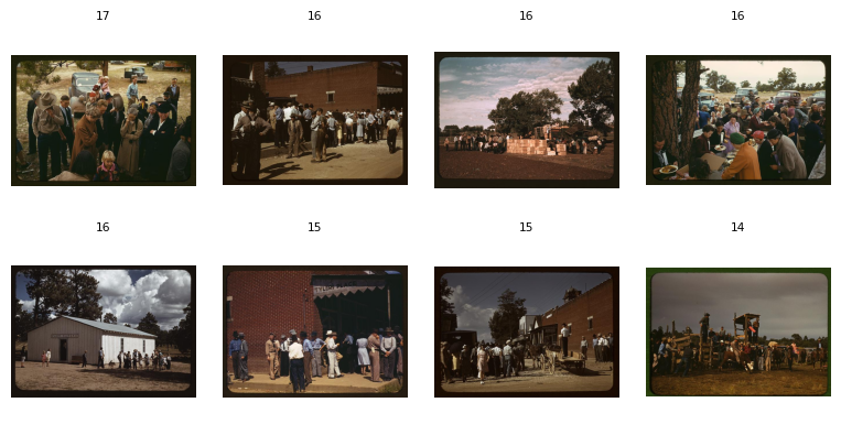
The model successfully identifies crowd scenes, though the exact count becomes less reliable as the number of people increases. In dense crowds, overlapping individuals and partial occlusions make precise counting challenging. Nevertheless, the detection provides a useful proxy for the scale of human presence in each photograph.
The number of people varies considerably by photographer, reflecting different documentary styles and subject matter choices.
(
    fsac
    .pipe(ggplot, aes("reorder(photographer, people)", "people"))
    + geom_boxplot()
    + coord_flip()
)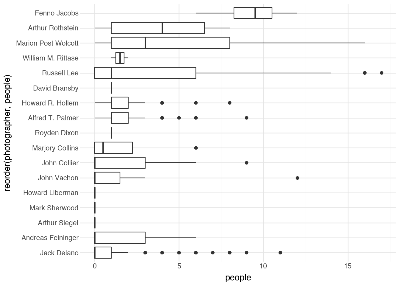
Some photographers specialized in intimate portraits with one or two subjects, while others captured street scenes and public gatherings. These patterns emerge clearly from the automated analysis.
20.8 Segmentation
Object detection tells us where objects are, but treats each detection as a simple rectangle. Instance segmentation goes further by identifying the exact pixels that belong to each object. Instead of a bounding box, segmentation produces a mask—a binary image where pixels belonging to the object are marked as 1 and background pixels as 0.
Segmentation models build on object detection architectures by adding a mask prediction branch. For each detected object, the model predicts not just a bounding box but also a pixel-wise mask within that box. The training loss includes an additional component for mask accuracy:
\[ \mathcal{L}_{\text{mask}} = -\frac{1}{N} \sum_{i=1}^{N} \left[ y_i \log(\hat{y}_i) + (1 - y_i) \log(1 - \hat{y}_i) \right] \]
This is the binary cross-entropy loss computed over all \(N\) pixels in the mask region, where \(y_i\) is the ground-truth label (1 if the pixel belongs to the object, 0 otherwise) and \(\hat{y}_i\) is the predicted probability. The loss penalizes both false positives (predicting object when the pixel is background) and false negatives (predicting background when the pixel is object).
YOLO includes segmentation variants that maintain real-time performance while producing pixel-accurate masks.
model = YOLO("yolo11n-seg.pt")
pred = model.predict("media/fsac/1a35210v.jpg")

rgb = cv2.cvtColor(pred[0].plot(), cv2.COLOR_BGR2RGB)
pil_img = Image.fromarray(rgb)
pil_img
image 1/1 /Users/admin/gh/fds-py/media/fsac/1a35210v.jpg: 544x640 3 persons, 36.0ms
Speed: 0.6ms preprocess, 36.0ms inference, 1.6ms postprocess per image at shape (1, 3, 544, 640)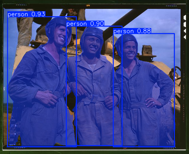
The visualization now shows colored masks overlaid on detected objects, precisely delineating their boundaries rather than just enclosing them in rectangles. This pixel-level precision enables more nuanced analysis of image content.
We can use segmentation to compute what percentage of each image is occupied by people, providing a measure of how prominently human figures feature in the composition.
results = []
for row in fsac.iter_rows(named=True):
    preds = model.predict(row["filepath"], verbose=False)[0]

    cls_ids = preds.boxes.cls.to("cpu").numpy().astype(int)
    names = preds.names

    person_idx = np.where(np.array([names[c] == "person" for c in cls_ids]))[0]
    if person_idx.size == 0:
        results.append(0.0)
        continue

    masks = preds.masks.data[person_idx]
    union = masks.any(dim=0)

    coverage = union.float().mean().item()
    results.append(coverage * 100)


fsac = fsac.with_columns(people_prop=pl.Series(results))
fsac
shape: (500, 4)
| filepath | photographer | people | people_prop |
|---|---|---|---|
| str | str | i64 | f64 |
| "media/fsac/1a35266v.jpg" | "Alfred T. Palmer" | 0 | 0.0 |
| "media/fsac/1a34940v.jpg" | "Howard R. Hollem" | 0 | 0.0 |
| "media/fsac/1a34143v.jpg" | "Russell Lee" | 10 | 3.520182 |
| "media/fsac/1a35375v.jpg" | "Alfred T. Palmer" | 1 | 19.758731 |
| "media/fsac/1a34758v.jpg" | "Jack Delano" | 0 | 0.0 |
| … | … | … | … |
| "media/fsac/1a34359v.jpg" | "Marion Post Wolcott" | 8 | 28.831056 |
| "media/fsac/1a34893v.jpg" | "Howard R. Hollem" | 1 | 8.354187 |
| "media/fsac/1a34100v.jpg" | "Russell Lee" | 1 | 3.764648 |
| "media/fsac/1a35045v.jpg" | "Howard Liberman" | 0 | 0.0 |
| "media/fsac/1a34863v.jpg" | "Howard R. Hollem" | 0 | 0.0 |
The people_prop column now contains the percentage of each image covered by detected people. Let’s see which images have the highest human coverage.
(
    fsac
    .sort(c.people_prop, descending=True)
    .head(8)
    .pipe(DSImage.plot_image_grid, ncol=4, label_name="people_prop")
)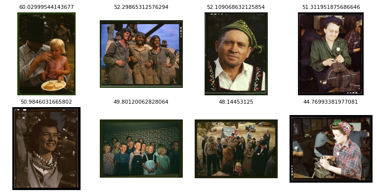
These tend to be closely framed portraits where the subject fills most of the frame. The segmentation-based measure captures a different aspect of photographic style than simple person counts: a single person in a tight portrait can have higher coverage than a dozen people in a wide street scene.
The relationship between person coverage and photographer reveals stylistic differences.
(
    fsac
    .group_by(c.photographer)
    .agg(avg_people = c.people_prop.mean())
    .pipe(ggplot, aes("avg_people", "reorder(photographer, avg_people)"))
    + geom_point()
)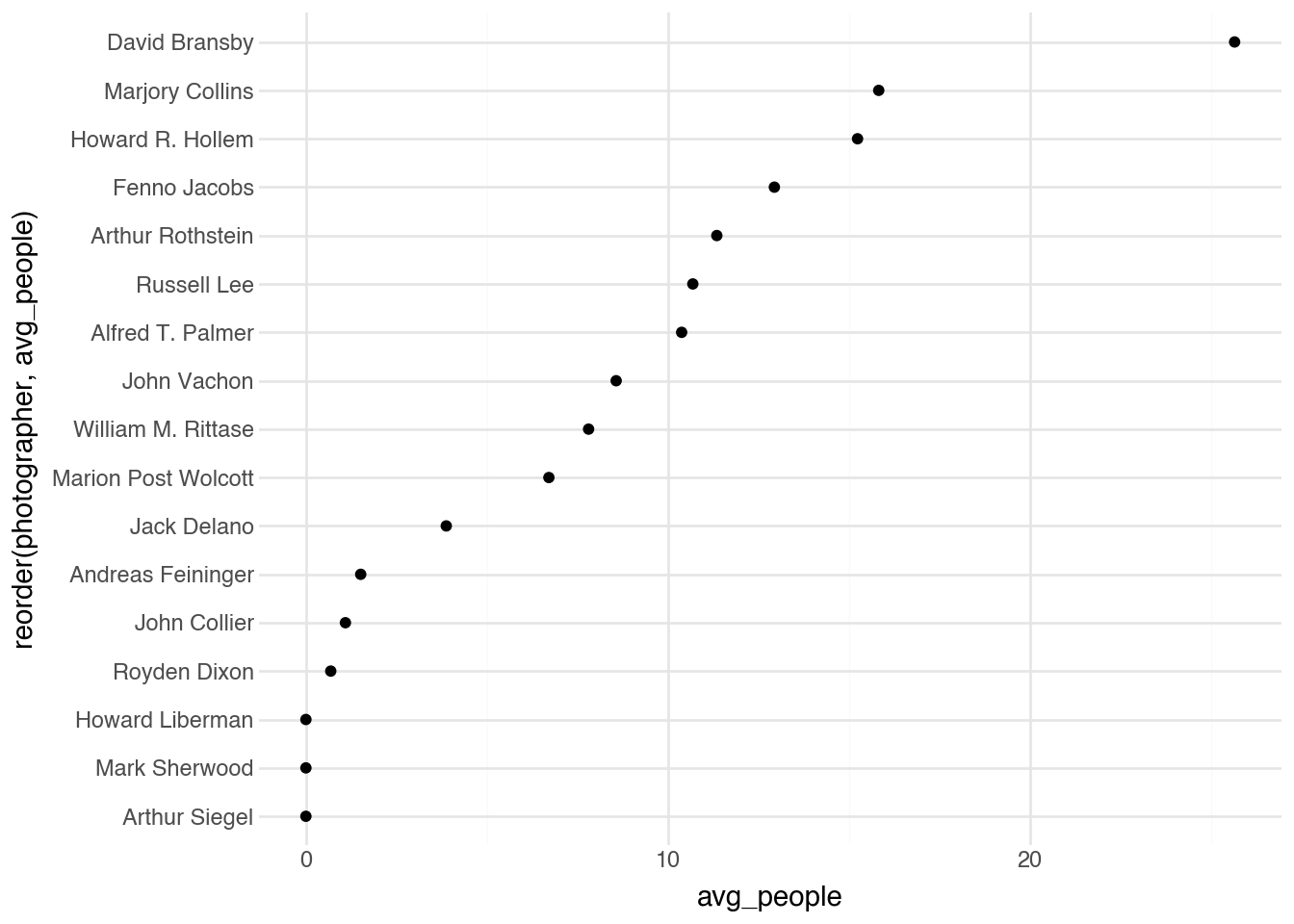
Photographers with higher average coverage tended toward portrait work, while those with lower coverage may have focused on environmental scenes, architecture, or wide-angle documentary shots. The measure is not always inversely related to person count; some photographers captured groups in intimate settings with high coverage, while others documented single individuals in expansive landscapes.
20.9 Pose Detection
Human pose estimation identifies the locations of body parts in an image, typically represented as a set of keypoints corresponding to joints like shoulders, elbows, wrists, hips, knees, and ankles. These keypoints, connected according to human anatomy, form a “skeleton” that describes body position and posture.
Pose estimation models predict coordinates for each keypoint along with confidence scores indicating detection reliability. The COCO pose format defines 17 keypoints: nose, left/right eyes, left/right ears, left/right shoulders, left/right elbows, left/right wrists, left/right hips, left/right knees, and left/right ankles.
The training loss for pose estimation typically combines localization accuracy with visibility prediction:
\[ \mathcal{L}_{\text{pose}} = \sum_{k=1}^{K} v_k \cdot \left\| \mathbf{p}_k - \hat{\mathbf{p}}_k \right\|^2 \]
where \(K\) is the number of keypoints, \(v_k\) is a visibility flag (1 if the keypoint is visible, 0 otherwise), \(\mathbf{p}_k\) is the ground-truth position, and \(\hat{\mathbf{p}}_k\) is the predicted position. This formulation only penalizes errors on visible keypoints, acknowledging that occluded body parts cannot be reliably localized.
Advanced pose estimation models use heatmap-based representations, predicting a probability distribution over possible keypoint locations:
\[ \mathcal{L}_{\text{heatmap}} = \sum_{k=1}^{K} \sum_{(x,y)} \left( H_k(x, y) - \hat{H}_k(x, y) \right)^2 \]
where \(H_k(x, y)\) is the ground-truth heatmap (typically a 2D Gaussian centered on the keypoint) and \(\hat{H}_k(x, y)\) is the predicted heatmap.
Let’s apply pose detection to our historical photographs.
model = YOLO("yolo11n-pose.pt")
pred = model.predict("media/fsac/1a35210v.jpg")


rgb = cv2.cvtColor(pred[0].plot(), cv2.COLOR_BGR2RGB)
pil_img = Image.fromarray(rgb)
pil_img
image 1/1 /Users/admin/gh/fds-py/media/fsac/1a35210v.jpg: 544x640 3 persons, 27.5ms
Speed: 0.5ms preprocess, 27.5ms inference, 0.3ms postprocess per image at shape (1, 3, 544, 640)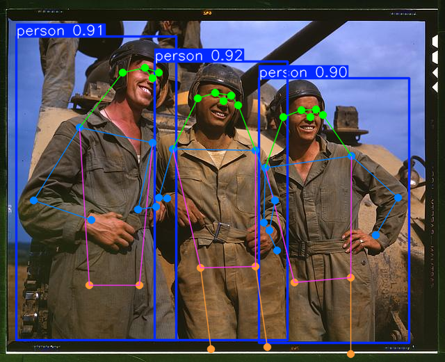
The visualization shows detected poses as skeleton overlays, with lines connecting keypoints according to anatomical structure. The colored points indicate individual keypoints, while the connecting lines show the body structure.
We can use pose information to analyze photographic composition in sophisticated ways. Let’s compute the proportion of image height occupied by the torso of the largest detected person. This metric indicates how prominently human figures are framed in each photograph.
results = []

for row in fsac.iter_rows(named=True):
    preds = model.predict(row["filepath"], verbose=False)[0]

    if preds.keypoints is None:
        results.append(0.0)
        continue

    img_h = preds.orig_img.shape[0]

    xy = preds.keypoints.xy
    conf = preds.keypoints.conf

    if conf is None:
        results.append(0.0)
        continue

    xy = xy.cpu().numpy()
    conf = conf.cpu().numpy()

    best_torso = 0.0

    for i in range(xy.shape[0]):
        kpt_confs = conf[i, [5, 6, 11, 12]]
        if np.any(kpt_confs < 0.5):
            continue

        mid_sh = xy[i, [5, 6], :].mean(axis=0)
        mid_hip = xy[i, [11, 12], :].mean(axis=0)

        torso_len = float(np.linalg.norm(mid_sh - mid_hip))

        if torso_len > best_torso:
            best_torso = torso_len

    torso_pct = (best_torso / img_h) * 100.0 if best_torso > 0 else 0.0
    results.append(torso_pct)

fsac = fsac.with_columns(torso=pl.Series(results))
fsac
shape: (500, 5)
| filepath | photographer | people | people_prop | torso |
|---|---|---|---|---|
| str | str | i64 | f64 | f64 |
| "media/fsac/1a35266v.jpg" | "Alfred T. Palmer" | 0 | 0.0 | 0.0 |
| "media/fsac/1a34940v.jpg" | "Howard R. Hollem" | 0 | 0.0 | 0.0 |
| "media/fsac/1a34143v.jpg" | "Russell Lee" | 10 | 3.520182 | 0.0 |
| "media/fsac/1a35375v.jpg" | "Alfred T. Palmer" | 1 | 19.758731 | 47.362576 |
| "media/fsac/1a34758v.jpg" | "Jack Delano" | 0 | 0.0 | 0.0 |
| … | … | … | … | … |
| "media/fsac/1a34359v.jpg" | "Marion Post Wolcott" | 8 | 28.831056 | 21.056602 |
| "media/fsac/1a34893v.jpg" | "Howard R. Hollem" | 1 | 8.354187 | 24.024989 |
| "media/fsac/1a34100v.jpg" | "Russell Lee" | 1 | 3.764648 | 11.063779 |
| "media/fsac/1a35045v.jpg" | "Howard Liberman" | 0 | 0.0 | 0.0 |
| "media/fsac/1a34863v.jpg" | "Howard R. Hollem" | 0 | 0.0 | 0.0 |
The computation identifies the shoulder and hip keypoints (indices 5, 6 for shoulders and 11, 12 for hips), calculates the midpoint of each pair, and measures the distance between them. This torso length, expressed as a percentage of image height, indicates how large human subjects appear in the frame.
(
    fsac
    .sort(c.torso, descending=True)
    .head(8)
    .pipe(DSImage.plot_image_grid, ncol=4, label_name="torso")
)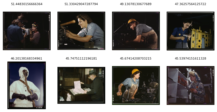
The images with the highest torso proportions are medium shots of workers and subjects, framed tightly enough that the torso occupies a substantial portion of the vertical space. These are neither extreme close-ups (which might exclude the torso entirely) nor distant shots (where the full figure would be small).
This metric shows strong variation by photographer.
(
    fsac
    .filter(c.torso > 0)
    .group_by(c.photographer)
    .agg(torso_mean = c.torso.mean(), n = pl.len())
    .filter(c.n > 0)
    .pipe(ggplot, aes("torso_mean", "reorder(photographer, torso_mean)"))
    + geom_point()
)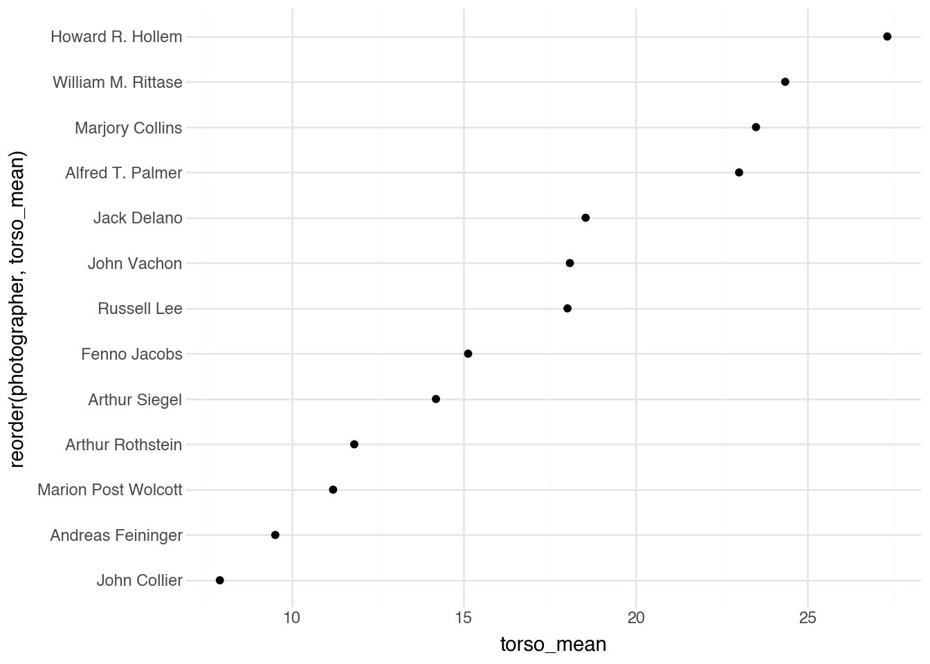
The differences reflect distinct documentary styles: some photographers favored intimate working shots that captured subjects at medium distance, while others preferred wider environmental compositions or tighter facial portraits. Pose estimation enables these nuanced analyses of compositional choices that would be difficult to quantify manually.
This approach could be extended in many directions: analyzing face orientation to study where subjects are looking, comparing the poses of multiple people to identify group dynamics, or tracking limb positions to characterize types of physical activity depicted in photographs.
20.10 Training YOLO
The pre-trained YOLO models we have used so far recognize objects from the COCO dataset: people, cars, dogs, and other common categories. But what if we want to detect objects specific to our domain? Training a custom YOLO model requires labeled data where humans have drawn bounding boxes around objects of interest and assigned class labels to each box.
Our bird bounding box dataset contains exactly this information. Each row specifies an image filepath, a species label, and four coordinates defining the corners of a bounding box around the bird.
birds_bbox
shape: (1_000, 7)
| label | filepath | bbox_x0 | bbox_y0 | bbox_x1 | bbox_y1 | index |
|---|---|---|---|---|---|---|
| str | str | f64 | f64 | f64 | f64 | str |
| "Gray_Catbird" | "media/birds_1000/00000.png" | 15.0 | 44.0 | 480.0 | 331.0 | "train" |
| "Sayornis" | "media/birds_1000/00001.png" | 131.0 | 85.0 | 488.0 | 326.0 | "train" |
| "Tennessee_Warbler" | "media/birds_1000/00002.png" | 40.0 | 5.0 | 345.0 | 239.0 | "test" |
| "White_throated_Sparrow" | "media/birds_1000/00003.png" | 99.0 | 42.0 | 448.0 | 344.0 | "train" |
| "Ring_billed_Gull" | "media/birds_1000/00004.png" | 104.0 | 32.0 | 451.0 | 284.0 | "train" |
| … | … | … | … | … | … | … |
| "White_breasted_Kingfisher" | "media/birds_1000/00995.png" | 17.0 | 105.0 | 419.0 | 336.0 | "test" |
| "Blue_Grosbeak" | "media/birds_1000/00996.png" | 96.0 | 102.0 | 361.0 | 338.0 | "test" |
| "Yellow_headed_Blackbird" | "media/birds_1000/00997.png" | 53.0 | 42.0 | 424.0 | 208.0 | "train" |
| "Tree_Sparrow" | "media/birds_1000/00998.png" | 47.0 | 11.0 | 450.0 | 427.0 | "train" |
| "Cliff_Swallow" | "media/birds_1000/00999.png" | 158.0 | 50.0 | 352.0 | 316.0 | "train" |
The bbox_x0 and bbox_y0 columns give the coordinates of the upper-left corner, while bbox_x1 and bbox_y1 give the lower-right corner. The index column indicates whether each image belongs to the training set or the test set, a split we made beforehand to enable honest evaluation of model performance.
YOLO expects training data in a specific directory structure with images and label files organized into train and validation folders. Our helper function DSImage.build_yolo_data converts our tabular format into the required layout, creating a YAML configuration file that tells YOLO where to find the data and what classes to recognize.
DSImage.prepare_yolo_dataset(
    birds_bbox, root="media/yolo_birds", yaml_name="birds.yaml"
)
With the data prepared, training proceeds by loading a pre-trained model and calling its train method. We start from yolo11n.pt, a model already trained on COCO, and fine-tune it on our bird data. This transfer learning approach leverages features the model has already learned from millions of general images, adapting them to our specific task.
model = YOLO("yolo11n.pt")
model.train(data="media/yolo_birds/birds.yaml", epochs=50, imgsz=640)
model.save("yolo_birds_final.pt")
The epochs parameter controls how many complete passes through the training data the model makes, with each epoch updating the model weights based on the loss function described earlier. The imgsz parameter specifies the image size used during training; images are resized to 640×640 pixels regardless of their original dimensions.
After training completes, we evaluate performance on the held-out test set using the val method. This computes standard object detection metrics that quantify how well the model’s predictions match ground-truth annotations.
metrics = model.val(data="media/yolo_birds/birds.yaml", imgsz=640)The primary metrics for object detection are variants of mean Average Precision (mAP), which measures how well the model balances finding all relevant objects (recall) with avoiding false detections (precision). To understand mAP, we first need to define when a predicted bounding box counts as a correct detection.
A prediction is considered a true positive if its Intersection over Union (IoU) with a ground-truth box exceeds some threshold. Recall that IoU measures the overlap between two boxes:
\[ \text{IoU} = \frac{\text{Area of Intersection}}{\text{Area of Union}} \]
An IoU of 1.0 means perfect overlap, while 0 means no overlap at all. The choice of IoU threshold determines how strict we are about localization accuracy. For each class, we can compute precision and recall at various confidence thresholds, tracing out a precision-recall curve. Average Precision (AP) summarizes this curve as the area underneath it:
\[ \text{AP} = \int_0^1 p(r) \, dr \]
where \(p(r)\) is precision at recall level \(r\). In practice, this integral is approximated by interpolating the precision-recall curve at discrete points. The mAP50 metric uses an IoU threshold of 0.50, meaning a prediction counts as correct if it overlaps with the ground truth by at least 50%. This is a relatively lenient standard that rewards finding objects even if the bounding box is not perfectly aligned.
metrics.box.map50The mAP50-95 averages performance across multiple IoU thresholds from 0.50 to 0.95 in steps of 0.05:
\[ \text{mAP50-95} = \frac{1}{10} \sum_{t \in \{0.50, 0.55, \ldots, 0.95\}} \text{mAP}_t \]
This stricter metric rewards precise localization. A model might achieve high mAP50 by finding objects with roughly correct boxes, but achieving high mAP50-95 requires tight alignment between predictions and ground truth.
metrics.box.mapThe gap between these two metrics reveals how well the model localizes objects. A large gap suggests the model finds objects but draws imprecise boxes; a small gap indicates accurate localization.
Finally, let’s see the trained model in action on a test image it has never seen during training.
path = birds_bbox.filter(c.index == "test").select(c.filepath.last()).item()
pred = model.predict(path)

rgb = cv2.cvtColor(pred[0].plot(), cv2.COLOR_BGR2RGB)
pil_img = Image.fromarray(rgb)
pil_img
image 1/1 /Users/admin/gh/fds-py/media/birds_1000/00996.png: 512x640 1 bird, 21.2ms
Speed: 1.0ms preprocess, 21.2ms inference, 0.3ms postprocess per image at shape (1, 3, 512, 640)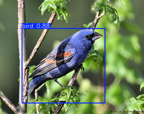
And, at least in this one example, it does a very good job of boxing in the bird within the image.
20.11 Vision Language Models
The models we have explored so far each produce structured outputs: bounding boxes, segmentation masks, or keypoint coordinates. These representations are useful for quantitative analysis but do not capture the full richness of what an image depicts. A photograph of workers in a factory contains not just “3 persons detected” but a story about labor, industry, and daily life. Extracting such narrative content has traditionally required human interpretation.
Vision Language Models (VLMs) bridge this gap by combining visual understanding with natural language generation. These models can look at an image and produce free-form text descriptions, answer questions about visual content, or engage in dialogue about what they see. They represent a convergence of computer vision and large language models, trained on massive datasets of images paired with textual descriptions.
The architecture of a VLM typically consists of three components: a vision encoder that processes the image into a sequence of visual tokens, a projection layer that maps these tokens into the same embedding space used by the language model, and a language model that generates text conditioned on both the visual tokens and any text prompt. During training, the model learns to associate visual patterns with their linguistic descriptions, enabling it to describe novel images it has never seen before.
VLMs open new possibilities for image analysis. Rather than counting objects or measuring pixel proportions, we can ask open-ended questions: “What activity is taking place in this photograph?” or “Describe the mood conveyed by this image.” The responses, while subjective and sometimes imperfect, capture aspects of visual content that structured outputs cannot represent.
Let’s use the OpenAI API to get a description of one of our FSA photographs. We will send the image to a vision-capable model and ask it to describe what it sees.
import base64
from openai import OpenAI

client = OpenAI()

image_path = "media/fsac/1a35210v.jpg"

with open(image_path, "rb") as f:
    image_data = base64.standard_b64encode(f.read()).decode("utf-8")

text = ("Provide a detailed plain-text description of the "
       "objects, activities, people, background and/or composition "
       "of this photograph")


response = client.chat.completions.create(
    model="gpt-5-mini-2025-08-07",
    messages=[
        {
            "role": "user",
            "content": [
                {
                    "type": "text",
                    "text": text
                },
                {
                    "type": "image_url",
                    "image_url": {
                        "url": f"data:image/jpeg;base64,{image_data}"
                    }
                }
            ]
        }
    ]
)

print(response.choices[0].message.content)
The photograph shows a close, waist-up group portrait of three young men in
military work clothes standing in front of an armored vehicle. Each man wears
a one-piece coverall or boiler suit, belted at the waist, and a padded tank
helmet with ear flaps or built-in headphones. Their coveralls are dusty and
stained with grease and dirt; their faces and hands also show grime,
suggesting recent hard work or field activity.  All three men are smiling
broadly and appear relaxed and friendly with one another. The central figure
stands slightly forward with his arms linked to the two men beside him; the
man on the left has one hand resting on his hip, and the man on the right has
a hand on his belt. Their posture and expressions convey camaraderie and a
moment of shared good spirits.  Behind them, a large tank or armored vehicle
dominates the background. The vehicle’s turret and a long gun barrel run
diagonally across the upper right of the image. Parts of the tank’s hull and
tracks are visible, showing a dusty, worn surface. In the upper left
background, a pair of legs and a boot belonging to another crew member can
be seen standing on the vehicle, only partially included in the frame.
The setting is outdoors under a clear blue sky; a low horizon of open
countryside or field is visible in the far background. The photograph is
in color with warm, natural daylight highlighting the men’s faces and the
textured surfaces of their clothing and the vehicle. The composition centers
the trio, creating a tight, informal group portrait against the larger
mechanical backdrop, emphasizing both the human element and the military
equipment. The image has the look of a candid, in-the-field moment rather
than a formal posed studio shot.
The model returns a natural language description that captures elements no structured detector could identify: the apparent era suggested by clothing and photographic style, the social context implied by the scene, and interpretive observations about mood or activity. This kind of output is inherently more subjective than counting bounding boxes, but it provides a different and complementary form of understanding.
VLMs can also be used programmatically to generate structured data from images. By carefully crafting prompts, you can ask the model to output JSON with specific fields, effectively creating a flexible object detector that can identify whatever categories you specify without retraining. This approach trades some accuracy for remarkable flexibility: the same model can describe fashion items, identify architectural styles, or catalog the contents of historical photographs.
The combination of structured computer vision models and flexible VLMs provides a powerful toolkit. Use object detection when you need precise counts and locations. Use segmentation when pixel-level boundaries matter. Use pose estimation for body position analysis. And use VLMs when you need rich, contextual descriptions or want to extract information that no pre-trained detector was designed to find.
20.12 Conclusions
This chapter has explored a range of techniques for extracting information from images, progressing from simple pixel statistics to sophisticated deep learning models and vision language models. Each approach offers different tradeoffs between interpretability, computational cost, and semantic richness.
Basic pixel-level features like brightness and color distributions are fast to compute and easy to understand. They capture global properties of images and can reveal interesting patterns across collections. However, these features cannot distinguish between a yellow bird and a yellow background, or between a dark subject and a dark photograph.
Deep learning models for object detection, segmentation, and pose estimation offer dramatically more sophisticated understanding. These models identify meaningful objects, delineate their boundaries at pixel precision, and localize body parts in complex poses. They enable analyses that would be impossible with simple features: counting people in crowds, measuring how much of an image depicts human figures, or characterizing body positions.
Vision language models add yet another dimension by producing natural language descriptions of visual content. They capture contextual and interpretive aspects of images that structured outputs cannot represent, though their outputs require different analytical approaches than numerical features.
Beyond the specific models explored here, remember that images can be converted to embeddings using transfer learning approaches (Chapter 15), enabling classification, clustering, and visualization with standard machine learning tools. This embedding-based approach is particularly valuable when your analytical categories don’t match the labels in pre-trained models.
The models we explored here—YOLO variants trained on the COCO dataset and VLMs trained on web-scale image-text pairs—represent just a sample of available approaches. The field of computer vision continues to advance rapidly, with new architectures and training techniques regularly improving accuracy and enabling new capabilities. The fundamental pattern, however, remains consistent: we extract information from images by combining low-level pixel data with learned representations that capture semantic meaning.
For data science applications, image analysis opens vast possibilities. Archives of historical photographs can be systematically analyzed to understand social patterns. Medical images can be screened for abnormalities. Satellite imagery can track environmental changes. Social media photographs can reveal trends in consumer behavior. Wherever images contain information, the techniques in this chapter provide tools to extract it.