1 + 12In this book, we focus on tools and techniques for exploratory data analysis, also known as EDA. Initially described in John Tukey’s classic text of the same name, EDA is a general approach to examining data through visualizations and broad summary statistics [1] [2]. It prioritizes studying data directly to generate hypotheses and ascertain general trends prior to and often in lieu of formal statistical modeling. The growth in both data volume and complexity has further increased the need for careful application of these exploratory techniques. In the intervening years, EDA techniques have become widely used within statistics, computer science, and many other data-driven fields and professions.
The histories of data programming and EDA are deeply entwined. Concurrent with Tukey’s development of exploratory data analysis (EDA), Rick Becker, John Chambers, and Allan Wilks of Bell Labs began developing software designed specifically for statistical computing. By 1980, the ‘S’ language was released for general distribution outside Bell Labs. It was followed by a popular series of books and updates, including ‘New S’ and ‘S-Plus’ [3] [4] [5] [6]. In the early 1990s, Ross Ihaka and Robert Gentleman produced a fully open-source implementation of S called ‘R’. The name ‘R’ was chosen both as a play on the previous letter in the alphabet and as a reference to the authors’ shared initial. Their implementation has become the de facto standard tool in statistics. More recently, many of R’s best ideas have been extended to other general-purpose programming languages such as Python and JavaScript.
The ideas and methods of exploratory data analysis (EDA) have been successfully adopted and extended in Python through a rich ecosystem of data science libraries. Python, originally created by Guido van Rossum in 1991, has evolved into one of the most popular programming languages for data analysis, machine learning, and scientific computing. Pandas, developed by Wes McKinney beginning in 2008, brought R-like data structures and manipulation capabilities to Python [7]. Matplotlib and, later, Seaborn provided comprehensive plotting capabilities, while plotnine implemented the grammar of graphics approach pioneered by ggplot2 in R. More recently, Polars has emerged as a high-performance alternative to pandas for large-scale data manipulation.
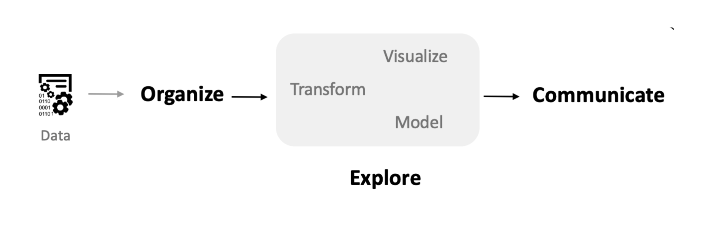
This Python ecosystem preserves the philosophy behind EDA: prioritizing interactive exploration, readable code, and the ability to move seamlessly between data manipulation, visualization, and analysis. We see this book as contributing to efforts to bring new communities into data analysis and to help shape that analysis by offering the humanities and humanistic social sciences powerful tools for data-driven inquiry. A visual summary of the steps of EDA is shown above in Fig. 1.1. We will see that the core chapters in this text map onto the steps outlined in the diagram.
While it is possible to read this book as a conceptual text, we expect that the majority of readers will eventually want to follow along with the code and examples given throughout the text. The first step is to obtain a working installation of Python with the necessary data science modules. For readers new to programming, we recommend getting started with Google Colab, which provides free access to a working Python session with no setup required. For users comfortable with the command line, the uv library is extremely powerful and reduces many of the pain points associated with other methods of setting up Python.
In addition to the Python software, following the examples in this text requires access to the datasets we use. Care has been taken to ensure that these are all in the public domain, making them easy to redistribute to readers. The materials and download instructions are available through the associated notebooks at the start of each chapter.
Learning to program is hard, and questions and issues will invariably arise in the process (even the most experienced users require help surprisingly frequently). As a first source of help, searching a question or error message in a search engine or a chat-based generative AI system will often pull up a solution directly related to your question. If you cannot find an immediate answer, the next best step is to find local, in-person help. While we’ve done our best in this static text to explain the concepts for working with Python, nothing beats talking to a real person.
The supplemental materials include all the data and code needed to replicate the analyses and visualizations in the book. We include the exact code that is printed in the book. We have used Quarto notebooks (with an .qmd extension) to store this code, with a file corresponding to each chapter. Quarto notebooks are an excellent choice for data analysis because they allow us to mix code, visualizations, and explanations within the same file. In fact, the entire data science workflow—from initial exploration through final presentation—can be contained within a single notebook. Furthermore, Quarto notebooks can be executed from Google Colab, allowing you to run the notebooks via a one-click link.
The Quarto environment provides a convenient way to view and edit notebooks. A notebook interface is organized into cells that contain either code or formatted text (markdown). Running a code cell executes the Python code and displays the output directly below the cell, making the environment ideal for exploratory data analysis because we can experiment and immediately see the results. Code cells typically have a gray background and can be executed by clicking the run button or pressing Shift+Enter. When we read or create a dataset, we can inspect it by typing the variable name in a cell.
Now let’s look at some examples of how to run Python code. In this book, we will show snippets of Python code and their output. Note that each snippet should be thought of as occurring in a code cell in a Quarto notebook. In one of its simplest forms, Python acts as a calculator. We can add 1 and 1 by typing 1 + 1 into a code cell; running the cell will display the output (2) below. In this book, we will present code and its output in a black box, with the Python code shown inside it and any output shown beneath. An example is given below.
1 + 12In addition to returning a value, running Python code can also store values by creating new variables. Variables in Python are used to store anything—such as numbers, datasets, functions, or models—that we want to use again later. Each variable has a name we can use to access it in later code. To create a variable, we use the = (equals) symbol, with the name on the left and the expression that produces the value on the right. For example, we can create a new variable called mynum with the value 8 by running the following code.
mynum = 3 + 5Notice that this code did not print any results because the result was saved to a new variable. We can now use our variable mynum in the same way we would use the number 8. For example, adding it to 1 yields the number nine:
mynum + 19Variable names must start with a letter or an underscore, but can contain numbers after the first character. We recommend using only lowercase letters and underscores. This makes it easier to read the code later without having to remember whether and where you used capital letters.
A function in Python takes a set of input values and returns an output value. Typically, a function has a format similar to the code below:
function_name(input1, input2)Where input1 and input2 are the values we pass to the first and second arguments of the function. The number of arguments is not always two, of course. There may be any number of arguments, including zero. There may also be additional optional arguments with default values that can be modified. Let us look at an example function: round. This function returns a rounded version of a number. If you give the function a single number, it returns the nearest integer. For example, here is the rounded value of π:
round(3.14159)3The function has an additional optional parameter that specifies the number of significant digits. For example, this will round π to two significant digits:
round(3.14159, 2)3.14An alternative way to call the same function is to use named arguments, where the two input values are specified by name rather than by position:
round(number=3.14159, ndigits=2)3.14How do we know the inputs to each function and what they do? In this text, we will explain the names and usage of the required inputs for new functions as they are introduced. To learn more about all of the possible inputs to a function, we can consult the function’s documentation. Python has excellent built-in documentation that can be accessed using the help() function. Most Python modules also have extensive online documentation. For example, the Polars library has comprehensive documentation at https://pola.rs/. We will learn how to use numerous functions in the coming chapters, each of which will help us explore and understand data.
A major selling point of Python is its extensive collection of user-contributed modules, available through the Python Package Index (PyPI). Most of the core modules we will need are already installed in Google Colab, and all we need to do is import them. When extra modules are needed, we will include lines of code such as the following to install them from within the Colab environment.
! pip install requests --quietOnce all modules are available, we’ll run code to load the modules we need into Python. Below is a common example of what we’ll have at the start of our scripts.
import numpy as np
import polars as pl

from funs import *
from plotnine import *
from polars import col as c
The lines that start with import make a module available for use in Python. Any function available within the module can be accessed by writing the module name followed by a dot and the function name. The as clauses create shortcuts that make the code easier to type. For example, after running the code above, we can call the read_csv function from Polars by typing pl.read_csv. Code that starts with from imports specific functions from the given libraries, making them available without needing to prefix them with the library name. The asterisk statements imports all the functions from the corresponding packages so you don’t have to import each one individually. The second-to-last line imports the col function from Polars and aliases it as c. We will use this function extensively throughout the book; the shorthand will greatly reduce clutter in our code. The final line loads all of the custom functions in a local file called funs.py. These are wrapper functions we have created to help simplify the code in this text. Each wrapper will be explained as they arise and can be directly inspected by opening the Python script directly.
In this book, we will be primarily working with data stored in a tabular format. Fig. 1.2 shows an example of a tabular dataset consisting of information about metropolitan regions in the United States. The figure shows structures organized by rows and columns. Each row of the dataset represents a particular metropolitan region; we call each row an observation. The columns represent the measurements we record for each observation; these measurements are called variables.
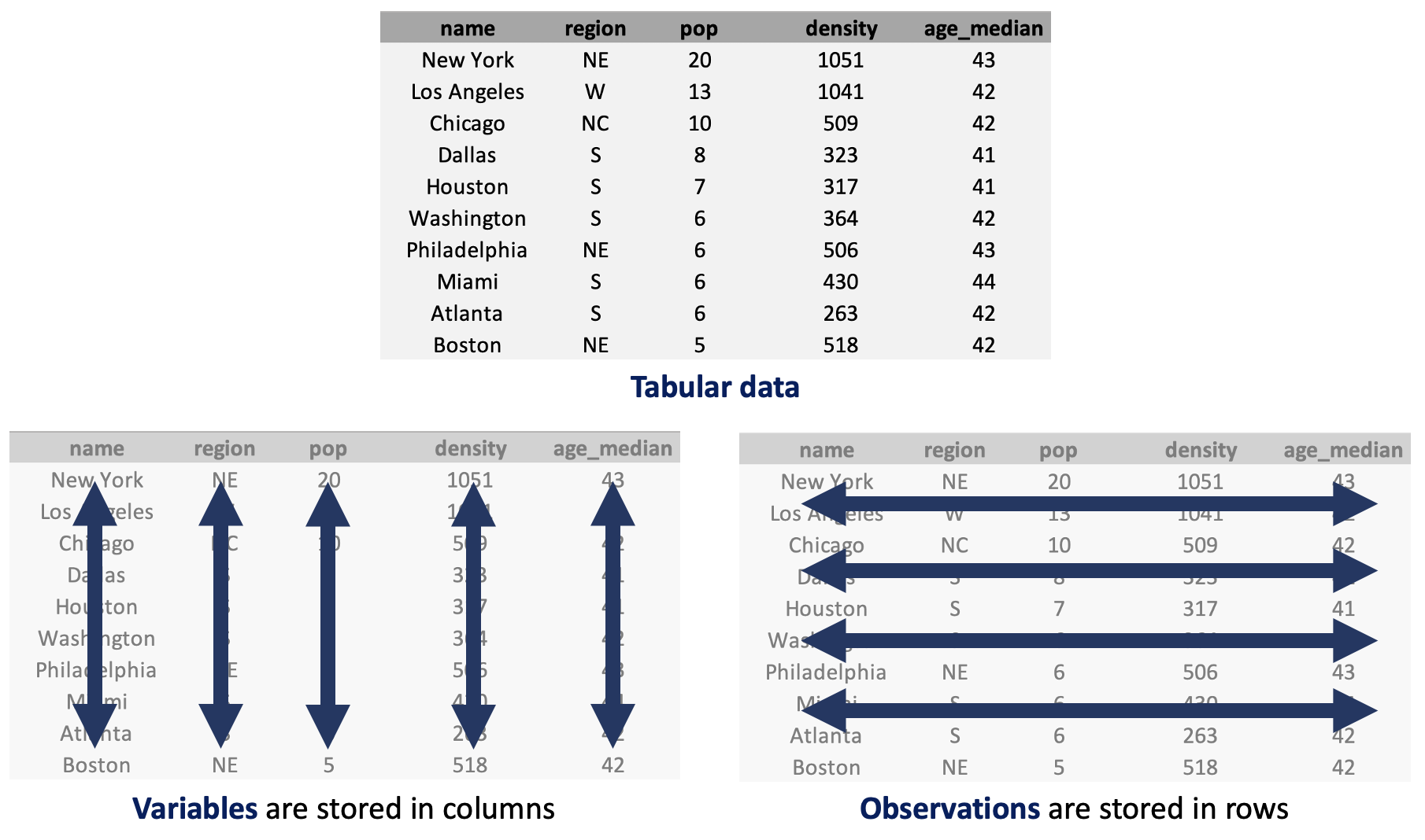
In our example dataset, we have five variables that record the region name, the quadrant of the country where the region is located, the region’s population (in millions), the population density (in tens of thousands of people per square kilometer), and the median age of the region’s residents. More details are given in the following section.
A common format for storing tabular datasets are in plaintext comma-separated values (CSV) files. Almost all of the datasets in this book will use this format for storing the data that we will work with. To read a dataset into Python, we use the function we use the function pl.read_csv() from the Polars library. We call pl.read_csv() with the path to the file relative to the script’s location. Below is an example of how to read the dataset contained in the file “data/countries.csv” and save it as an object called country. The resulting dataset is stored as a Python object called a DataFrame.
country = pl.read_csv("data/countries.csv")
country| iso | full_name | region | subregion | pop | lexp | lat | lon | hdi | gdp | gini | happy | cellphone | water_access | lang |
|---|---|---|---|---|---|---|---|---|---|---|---|---|---|---|
| str | str | str | str | f64 | f64 | f64 | f64 | f64 | i64 | f64 | f64 | f64 | f64 | str |
| "SEN" | "Senegal" | "Africa" | "Western Africa" | 18.932 | 70.43 | 14.366667 | -14.283333 | 0.53 | 4871 | 38.1 | 50.93 | 66.0 | 54.93987 | "pbp|fra|wol" |
| "VEN" | "Venezuela, Bolivarian Republic… | "Americas" | "South America" | 28.517 | 76.18 | 8.0 | -67.0 | 0.709 | 8899 | 44.8 | 57.65 | 96.8 | 95.66913 | "spa|vsl" |
| "FIN" | "Finland" | "Europe" | "Northern Europe" | 5.623 | 82.84 | 65.0 | 27.0 | 0.948 | 57574 | 27.7 | 76.99 | 156.4 | 99.44798 | "fin|swe" |
| "USA" | "United States of America" | "Americas" | "Northern America" | 347.276 | 79.83 | 39.828175 | -98.5795 | 0.938 | 78389 | 47.7 | 65.21 | 91.7 | 99.72235 | "eng" |
| "LKA" | "Sri Lanka" | "Asia" | "Southern Asia" | 23.229 | 78.51 | 7.0 | 81.0 | 0.776 | 14380 | 39.3 | 36.02 | 83.1 | 90.77437 | "sin|sin|tam|tam" |
| … | … | … | … | … | … | … | … | … | … | … | … | … | … | … |
| "ALB" | "Albania" | "Europe" | "Southern Europe" | 2.772 | 79.67 | 41.0 | 20.0 | 0.81 | 20362 | 30.8 | 54.45 | 91.9 | 98.5473 | "sqi" |
| "MYS" | "Malaysia" | "Asia" | "South-eastern Asia" | 35.978 | 76.03 | 3.7805111 | 102.314362 | 0.819 | 35990 | 46.2 | 58.68 | 118.2 | 95.69194 | "msa" |
| "SLV" | "El Salvador" | "Americas" | "Central America" | 6.366 | 76.98 | 13.668889 | -88.866111 | 0.678 | 12221 | 38.3 | 64.82 | 126.9 | 86.19786 | "spa" |
| "CYP" | "Cyprus" | "Asia" | "Western Asia" | 1.371 | 81.77 | 35.0 | 33.0 | 0.913 | 55720 | 31.2 | 60.71 | 123.1 | 99.41781 | "ell|tur" |
| "PAK" | "Pakistan" | "Asia" | "Southern Asia" | 255.22 | 66.71 | 30.0 | 71.0 | 0.544 | 5717 | 29.6 | 45.49 | 49.8 | 61.92651 | "eng|urd" |
Notice that the display shows a total of 135 rows and 15 columns. Or, with our terms defined above, there are 135 observations and 15 variables. Only the first five and last five observations are shown in the output, along with information about the shape of the DataFrame.
The data types shown by pandas tell us the types of data stored in each column. Here we see the three most common types: str (strings), i64 (integers; whole numbers stored in 64 bits), and f64 (floats; numbers with decimal points, also stored in 64 bits). We will refer to any variable of either integer or float type as numeric data. Knowing the data types of each column is important because, as we will see throughout the book, they affect the kinds of visualizations and analyses that can be applied. The data types in the DataFrame are automatically determined by the pl.read_csv() function. Optional arguments, such as dtype, can be used to specify alternatives, or we can modify data types after the DataFrame is created using techniques shown in the following chapters.
Throughout this book, we will use various datasets to illustrate concepts and show how each approach can be applied across different application domains. A complete description of all of the datasets used in the text and exercises can be found in Chapter 22. These include the variable names, types, sources, and some motivation behind each within the text.
In the following chapters, we will introduce the core concepts of exploratory data analysis relying heavily on the country dataset defined in which we have various pieces of metadata related to countries across the world. There are several associated datasets that we will also work with to illustrate additional concepts that are not directly applicable to the country-level data.
It is important to format Python code consistently. Even if code runs without errors and produces the desired results, consistent formatting makes it easier to read, debug, and maintain. Throughout this book, we will follow the conventions below, based on PEP 8 (Python’s official style guide). These are the same conventions used by professional data scientists and software developers. Adopt these rules whenever you write code for this course.
= and around binary operators (such as +, -, *, /, %, <, >, ==).def f(x=5): or geom_text(size=6))."hello" rather than 'hello').The following example applies these formatting rules in practice. Do not worry if you have not yet seen these specific functions or libraries; we will cover them later in the course. For now, focus on the structure and layout of the code.
(
    country
    .filter(c.region == "Europe")
    .pipe(ggplot, aes("hdi", "happy"))
    + geom_point()
    + geom_text(aes(label="iso"), size=6, nudge_y=0.5)
)
Notice how spacing, indentation, and line breaks work together to make the logic clear and readable. Following these conventions from the start will make your work easier to read, debug, and maintain.
Each chapter in this book contains a short concluding section with extensions to the main material. These include references for further study, additional Python libraries, and other suggested methods that may be of interest for the study of each specific type of humanities data.
In this chapter, we mention a few standard Python references that may be useful to consult alongside our text. The classic introduction to the Python language is Learning Python by Mark Lutz [8]. For those specifically interested in data science applications, Python for Data Analysis by Wes McKinney (the creator of pandas) provides comprehensive coverage of the core data science libraries [7].
For the specific approach to data analysis we follow in this book, Python Data Science Handbook by Jake VanderPlas is an excellent reference [9]. It covers the full stack of data science tools in Python, from basic data manipulation through machine learning. The book is also freely available online.
For those interested in the grammar of graphics approach to visualization that we use throughout this book, The Grammar of Graphics by Leland Wilkinson provides the theoretical foundation [10]. The plotnine module implements these concepts in Python, closely following the ggplot2 implementation in R.