import numpy as np
import polars as pl

from funs import *
from plotnine import *
from polars import col as c
theme_set(theme_minimal())

country = pl.read_csv("data/countries.csv")11 Supervised Learning
11.1 Setup
Load all of the modules and datasets needed for the chapter.
11.2 Introduction
The previous chapter introduced statistical inference, a set of methods for drawing conclusions about populations based on samples. In that context, the primary goal was understanding relationships between variables: determining whether differences between groups are statistically significant, whether two categorical variables are associated, or whether changes in one numerical variable are related to changes in another. Hypothesis tests and confidence intervals provided the framework for making such claims while accounting for sampling variability.
In this chapter, we shift our focus from inference to prediction. Rather than asking whether a relationship exists, we ask: given what we know about some variables, how well can we predict the value of another variable? This is the domain of supervised learning, a collection of methods designed to learn patterns from data that can be applied to make predictions on new, unseen observations.
The distinction between inference and prediction is subtle but important. In statistical inference, we typically care about the parameters of a model — the estimated coefficients, their standard errors, and their statistical significance. We ask questions like “Is there evidence that height is associated with driving speed?” In predictive modeling, we care primarily about the accuracy of predictions — how close our predicted values are to the actual values. We ask questions like “Given a student’s height and sex, what driving speed would we predict?” A model that performs well for inference may not perform well for prediction, and vice versa.
The term “supervised” in supervised learning refers to the fact that we train our models using data where the correct answers are already known. We have a set of input variables (called predictors, features, or independent variables) and an output variable (called the response, target, or dependent variable). The model learns from examples where both the inputs and outputs are observed, and then applies what it has learned to make predictions for cases where only the inputs are known.
This chapter introduces the fundamental concepts and techniques of supervised learning, beginning with the distinction between regression and classification problems. We will revisit linear regression from a predictive perspective, explore regularization techniques that improve prediction accuracy, and introduce gradient boosting as a powerful alternative to linear models. Throughout, we emphasize the importance of evaluating models on data they have not seen during training, a principle that separates predictive modeling from the descriptive statistics we have encountered earlier.
11.3 Predictive Modeling
The goal of predictive modeling is to generate predictions for one column in a dataset using information contained in one or more other columns. This might seem paradoxical at first: why would we want to predict values that we already have? The answer is that our ultimate goal is to apply the model to new data where the predictors are known but the value we want to predict is not. A hospital might use patient characteristics to predict the likelihood of readmission; a retailer might use purchase history to predict future spending; a researcher might use environmental measurements to predict species abundance. In each case, the model is trained on historical data where outcomes are known and then applied to future cases where outcomes have not yet occurred.
There are several types of predictive models, distinguished primarily by the data type of the variable being predicted. When we predict a numeric variable, the task is called regression. The name comes from the statistical technique of linear regression, though the term now encompasses many methods beyond simple linear models. When we predict a categorical variable — assigning observations to discrete groups or classes — the task is called classification. These two tasks require different evaluation criteria because the nature of prediction errors differs fundamentally between them.
For regression problems, we need a way to measure how far our predictions are from the actual values. The most common measure is the mean squared error (MSE), which computes the average of the squared differences between predicted and actual values. If we denote the actual values as \(y_1, y_2, \ldots, y_n\) and the corresponding predictions as \(\hat{y}_1, \hat{y}_2, \ldots, \hat{y}_n\), the MSE is defined as follows.
\[ \text{MSE} = \frac{1}{n} \sum_{i=1}^{n} (y_i - \hat{y}_i)^2 \]
Squaring the differences ensures that positive and negative errors do not cancel each other out and gives greater weight to larger errors. A model that makes occasional large mistakes will have a higher MSE than one that makes consistent small mistakes, even if the average error magnitude is similar.
Because the MSE is expressed in squared units of the response variable, it can be difficult to interpret directly. The root mean squared error (RMSE) addresses this by taking the square root of the MSE, returning the measure to the original units.
\[ \text{RMSE} = \sqrt{\text{MSE}} = \sqrt{\frac{1}{n} \sum_{i=1}^{n} (y_i - \hat{y}_i)^2} \]
The RMSE can be interpreted as the typical magnitude of prediction errors. An RMSE of 5 years in predicting life expectancy means that predictions are typically off by about 5 years in either direction.
For classification problems, the most straightforward measure of performance is the error rate, which simply counts the proportion of predictions that are incorrect. If we make \(n\) predictions and \(m\) of them are wrong, the error rate is \(m/n\). Equivalently, the accuracy is \((n-m)/n\), the proportion of correct predictions.
\[ \text{Error Rate} = \frac{\text{Number of incorrect predictions}}{\text{Total number of predictions}} \]
While the error rate provides a simple summary, it can be misleading in certain situations. If we are predicting a rare outcome — such as whether a patient has a rare disease — a model that always predicts “no disease” might have a very low error rate while being completely useless for its intended purpose. More sophisticated evaluation measures exist for such situations, but the error rate remains a useful starting point for understanding classification performance.
The process of building a predictive model is called training. During training, we use existing data to find parameter values that minimize prediction error. The general approach involves defining a model with numerical parameters — such as the coefficients in a linear regression — and then using optimization techniques to find the parameter values that produce the best predictions on the training data.
We encountered this idea in Chapter 10 when fitting linear regression models. The ordinary least squares method finds the intercept and slope values that minimize the sum of squared residuals. Predictive modeling extends this principle to a wide variety of model types, many of which require more sophisticated optimization techniques than simple calculus.
After training a model, we must evaluate how well it performs. A natural approach would be to compare predictions to the actual values in our data and compute the MSE or error rate. However, this approach has a fundamental flaw: the model was optimized specifically to fit this data, so its performance on this data will be overly optimistic.
Consider an extreme example. If we had a model flexible enough to memorize every observation in our dataset, it could achieve perfect predictions on that data — zero MSE, zero error rate. Yet such a model would be useless for predicting new observations because it has learned nothing general about the relationships in the data. It has simply memorized the answers.
This problem is called overfitting, and it represents one of the central challenges in predictive modeling. A model that fits the training data too closely captures not only the true underlying patterns but also the random noise specific to that particular sample. When applied to new data, the noise patterns will be different, and the model’s performance will suffer.
The solution is to evaluate models on data they have not seen during training. We create two subsets of our data: a training dataset used to fit the model and a testing dataset used to evaluate performance. The model is trained using only the training data, and then predictions are made for the testing data. The MSE or error rate computed on the testing set — called the test error — provides a more realistic assessment of how the model will perform on new observations.
Typically, we randomly assign observations to training and testing sets, often using proportions like 80 percent training and 20 percent testing. This random split ensures that both sets are representative of the overall data. Some situations require more careful splitting — for example, when data have a time component, we might train on earlier observations and test on later ones — but random splitting is a reasonable default for many applications.
11.4 Linear Regression Revisited
Having established the framework for predictive modeling, we can now revisit linear regression from a new perspective. In Chapter 10, we used linear regression primarily for inference: testing whether coefficients were significantly different from zero, constructing confidence intervals, and interpreting the relationships between variables. Here, we focus on prediction: how well can a linear model predict new observations?
The mathematical form of linear regression remains the same. Given a response variable \(y\) and predictor variables \(x_1, x_2, \ldots, x_k\), we model the relationship as:
\[ y = \alpha + \beta_1 x_1 + \beta_2 x_2 + \cdots + \beta_k x_k + \varepsilon \]
The coefficients \(\alpha\) and \(\beta_1, \ldots, \beta_k\) are estimated by minimizing the sum of squared residuals on the training data. Once these coefficients are estimated, we can make predictions for any observation by plugging in the predictor values and computing the predicted response.
To fit predictive models, we will use a class called DSSklearn, which provides a consistent interface to the scikit-learn machine learning library in Python. Like the DSStatsmodels class from the previous chapter, DSSklearn is designed to work within a Polars pipe chain. It takes as arguments the target variable (the column to predict) and a list of features (the columns to use as predictors).
model = (
    country
    .pipe(
        DSSklearn.linear_regression,
        target=c.lexp,
        features=[c.hdi, c.gdp, c.cellphone, c.happy]
    )
)
This code fits a linear regression model predicting life expectancy (lexp) using four predictors: the Human Development Index (hdi), GDP per capita (gdp), cellphone subscriptions per 100 people (cellphone), and a happiness index (happy). The function automatically splits the data into training and testing sets, fits the model on the training data, and stores everything needed to evaluate and use the model.
The resulting model object provides several methods for examining the results. The score method returns a dictionary containing the RMSE for both the training and testing sets.
model.score(){'train': np.float64(2.916788304946737), 'test': np.float64(3.103181695026965)}The training RMSE tells us how well the model fits the data it was trained on, while the testing RMSE provides a more realistic estimate of prediction accuracy on new data. A large gap between training and testing RMSE can indicate overfitting — the model has learned patterns specific to the training data that do not generalize well.
The coef method returns a DataFrame containing the estimated coefficients for each predictor.
model.coef()
shape: (5, 2)
| name | param |
|---|---|
| str | f64 |
| "Intercept" | 75.147766 |
| "hdi" | 6.061369 |
| "happy" | 0.859377 |
| "gdp" | -0.041938 |
| "cellphone" | -0.696483 |
These coefficients have the same interpretation as in the inferential context: each coefficient represents the expected change in the response for a one-unit change in the corresponding predictor, holding all other predictors constant. However, in the predictive context, we are less concerned with testing whether these coefficients are significantly different from zero and more concerned with whether they collectively produce accurate predictions.
The predict method returns a DataFrame with columns indicating whether each observation was in the training or testing set (index_), the actual response value (target_), and the model’s prediction (prediction_).
model.predict()
shape: (135, 3)
| index_ | target_ | prediction_ |
|---|---|---|
| str | f64 | f64 |
| "train" | 70.43 | 66.342595 |
| "train" | 76.18 | 73.382149 |
| "test" | 82.84 | 83.170286 |
| "train" | 79.83 | 82.999008 |
| "train" | 78.51 | 74.634218 |
| … | … | … |
| "train" | 79.67 | 77.20665 |
| "test" | 76.03 | 77.392255 |
| "train" | 76.98 | 72.158468 |
| "train" | 81.77 | 81.14838 |
| "train" | 66.71 | 66.771474 |
This output allows us to examine individual predictions and understand where the model performs well or poorly. We can also add the predictions to the original data using the with_columns method.
(
    country
    .with_columns(
        model.predict()
    )
)
shape: (135, 18)
| iso | full_name | region | subregion | pop | lexp | lat | lon | hdi | gdp | gini | happy | cellphone | water_access | lang | index_ | target_ | prediction_ |
|---|---|---|---|---|---|---|---|---|---|---|---|---|---|---|---|---|---|
| str | str | str | str | f64 | f64 | f64 | f64 | f64 | i64 | f64 | f64 | f64 | f64 | str | str | f64 | f64 |
| "SEN" | "Senegal" | "Africa" | "Western Africa" | 18.932 | 70.43 | 14.366667 | -14.283333 | 0.53 | 4871 | 38.1 | 50.93 | 66.0 | 54.93987 | "pbp|fra|wol" | "train" | 70.43 | 66.342595 |
| "VEN" | "Venezuela, Bolivarian Republic… | "Americas" | "South America" | 28.517 | 76.18 | 8.0 | -67.0 | 0.709 | 8899 | 44.8 | 57.65 | 96.8 | 95.66913 | "spa|vsl" | "train" | 76.18 | 73.382149 |
| "FIN" | "Finland" | "Europe" | "Northern Europe" | 5.623 | 82.84 | 65.0 | 27.0 | 0.948 | 57574 | 27.7 | 76.99 | 156.4 | 99.44798 | "fin|swe" | "test" | 82.84 | 83.170286 |
| "USA" | "United States of America" | "Americas" | "Northern America" | 347.276 | 79.83 | 39.828175 | -98.5795 | 0.938 | 78389 | 47.7 | 65.21 | 91.7 | 99.72235 | "eng" | "train" | 79.83 | 82.999008 |
| "LKA" | "Sri Lanka" | "Asia" | "Southern Asia" | 23.229 | 78.51 | 7.0 | 81.0 | 0.776 | 14380 | 39.3 | 36.02 | 83.1 | 90.77437 | "sin|sin|tam|tam" | "train" | 78.51 | 74.634218 |
| … | … | … | … | … | … | … | … | … | … | … | … | … | … | … | … | … | … |
| "ALB" | "Albania" | "Europe" | "Southern Europe" | 2.772 | 79.67 | 41.0 | 20.0 | 0.81 | 20362 | 30.8 | 54.45 | 91.9 | 98.5473 | "sqi" | "train" | 79.67 | 77.20665 |
| "MYS" | "Malaysia" | "Asia" | "South-eastern Asia" | 35.978 | 76.03 | 3.7805111 | 102.314362 | 0.819 | 35990 | 46.2 | 58.68 | 118.2 | 95.69194 | "msa" | "test" | 76.03 | 77.392255 |
| "SLV" | "El Salvador" | "Americas" | "Central America" | 6.366 | 76.98 | 13.668889 | -88.866111 | 0.678 | 12221 | 38.3 | 64.82 | 126.9 | 86.19786 | "spa" | "train" | 76.98 | 72.158468 |
| "CYP" | "Cyprus" | "Asia" | "Western Asia" | 1.371 | 81.77 | 35.0 | 33.0 | 0.913 | 55720 | 31.2 | 60.71 | 123.1 | 99.41781 | "ell|tur" | "train" | 81.77 | 81.14838 |
| "PAK" | "Pakistan" | "Asia" | "Southern Asia" | 255.22 | 66.71 | 30.0 | 71.0 | 0.544 | 5717 | 29.6 | 45.49 | 49.8 | 61.92651 | "eng|urd" | "train" | 66.71 | 66.771474 |
This combined DataFrame makes it easy to compare predictions to actual values while also seeing all the original variables, which can help diagnose why certain predictions are more or less accurate.
11.5 Lasso Regression
Linear regression estimates coefficients by minimizing the sum of squared residuals on the training data. While this produces the best possible fit to the training data, it does not necessarily produce the best predictions on new data. When models have many predictors, or when predictors are highly correlated with each other, the estimated coefficients can become unstable — small changes in the training data lead to large changes in the coefficients. This instability often leads to poor predictions on new observations.
Regularization addresses this problem by adding a penalty term to the optimization objective. Instead of simply minimizing squared residuals, we minimize squared residuals plus a penalty that discourages extreme coefficient values. This produces coefficients that are somewhat worse at fitting the training data but often better at predicting new data.
The lasso (Least Absolute Shrinkage and Selection Operator) is one of the most important regularization techniques. It adds a penalty proportional to the sum of the absolute values of the coefficients. If we denote the coefficients as \(\beta_1, \beta_2, \ldots, \beta_k\), the lasso objective function can be written as follows:
\[ \min_{\alpha, \beta} \left[ \sum_{i=1}^{n} (y_i - \alpha - \beta_1 x_{i1} - \cdots - \beta_k x_{ik})^2 + \lambda \sum_{j=1}^{k} |\beta_j| \right] \]
The parameter \(\lambda\) (lambda) controls the strength of the penalty. When \(\lambda = 0\), the lasso is equivalent to ordinary linear regression. As \(\lambda\) increases, the penalty term becomes more important, and coefficients are pushed toward zero. A remarkable property of the lasso is that it can push some coefficients exactly to zero, effectively removing those predictors from the model. This makes the lasso useful not only for improving predictions but also for variable selection — identifying which predictors are most important.
Why the Absolute Value?
The absolute value penalty is what gives the lasso its variable selection property. To understand why, imagine the optimization process searching for the best coefficients. When a coefficient is small, the absolute value penalty creates a constant “pull” toward zero, regardless of the coefficient’s current value. This pull can overcome the slight improvement in fit that a small coefficient provides, driving the coefficient all the way to zero. In contrast, other penalty forms (like the squared penalty used in ridge regression) create a pull that weakens as the coefficient approaches zero, so coefficients shrink but never quite reach zero.
Choosing the right value of \(\lambda\) is crucial. Too small a value provides little regularization and does not address overfitting; too large a value over-penalizes the coefficients and produces a model that underfits the data. Cross-validation is the standard approach for selecting \(\lambda\). The training data is divided into several folds (subsets), and for each candidate value of \(\lambda\), the model is trained on some folds and evaluated on the remaining fold. This process is repeated for all possible fold arrangements, and the \(\lambda\) value that produces the best average performance is selected.
The DSSklearn class handles cross-validation automatically when using the elastic_net_cv method, which is a general framework that includes the lasso as a special case. Setting l1_ratio=1 specifies that we want the lasso penalty.
model = (
    country
    .pipe(
        DSSklearn.elastic_net_cv,
        target=c.lexp,
        features=[c.hdi, c.gdp, c.cellphone, c.happy],
        l1_ratio=1
    )
)
The resulting model object provides the same methods as before. The score method shows performance on training and testing sets.
model.score(){'train': np.float64(2.961003671269824),
'test': np.float64(3.0813582323445163)}The predict method returns predictions.
model.predict()
shape: (135, 3)
| index_ | target_ | prediction_ |
|---|---|---|
| str | f64 | f64 |
| "train" | 70.43 | 66.86029 |
| "train" | 76.18 | 73.598074 |
| "test" | 82.84 | 83.095582 |
| "train" | 79.83 | 82.16778 |
| "train" | 78.51 | 74.952659 |
| … | … | … |
| "train" | 79.67 | 77.061804 |
| "test" | 76.03 | 77.588752 |
| "train" | 76.98 | 72.834118 |
| "train" | 81.77 | 81.054559 |
| "train" | 66.71 | 67.098843 |
The coef method shows the estimated coefficients.
model.coef()
shape: (5, 2)
| name | param |
|---|---|
| str | f64 |
| "Intercept" | 75.147766 |
| "hdi" | 5.487217 |
| "happy" | 0.5501 |
| "gdp" | 0.0 |
| "cellphone" | -0.0 |
Notice that some coefficients may be exactly zero or very close to zero, reflecting the lasso’s variable selection property. The model has determined that these predictors do not contribute enough to predictions to justify keeping them.
To compare the relative importance of predictors, it is helpful to examine coefficients on a standardized scale. The raw=True argument returns coefficients based on standardized (scaled) features, making the magnitudes comparable across predictors with different units.
model.coef(raw=True)
shape: (5, 2)
| name | param |
|---|---|
| str | f64 |
| "Intercept" | 45.41005 |
| "hdi" | 35.826175 |
| "happy" | 0.048348 |
| "gdp" | 0.0 |
| "cellphone" | -0.0 |
The alpha method returns the value of \(\lambda\) (called alpha in scikit-learn) selected by cross-validation.
model.alpha()np.float64(0.24888744821240497)Once we have identified the optimal penalty strength through cross-validation, we can refit the model with this specific value using elastic_net instead of elastic_net_cv. This is useful when we want more control over the fitting process.
(
    country
    .pipe(
        DSSklearn.elastic_net,
        target=c.lexp,
        features=[c.hdi, c.gdp, c.cellphone, c.happy],
        l1_ratio=1,
        alpha=1
    )
    .coef(raw=True)
    .filter(c.param != 0)
)
shape: (3, 2)
| name | param |
|---|---|
| str | f64 |
| "Intercept" | 49.565524 |
| "hdi" | 33.071864 |
| "happy" | 0.011268 |
The filter method selects only predictors with nonzero coefficients, showing us which variables the lasso has retained in the model.
11.6 Ridge Regression and ENet
While the lasso uses an absolute value penalty, ridge regression uses a squared penalty on the coefficients. The ridge objective function is:
\[ \min_{\alpha, \beta} \left[ \sum_{i=1}^{n} (y_i - \alpha - \beta_1 x_{i1} - \cdots - \beta_k x_{ik})^2 + \lambda \sum_{j=1}^{k} \beta_j^2 \right] \]
The squared penalty shrinks coefficients toward zero but, unlike the lasso, never shrinks them exactly to zero. This means ridge regression keeps all predictors in the model but with reduced influence. Ridge regression is particularly useful when predictors are highly correlated with each other, a situation where ordinary least squares and even the lasso can produce unstable estimates.
The elastic net combines both penalties, allowing the user to balance the lasso’s variable selection with ridge regression’s stability. The l1_ratio parameter controls this balance: a value of 1 gives the lasso (all absolute value penalty), a value of 0 gives ridge regression (all squared penalty), and intermediate values give a blend.
To fit a ridge regression model, we set l1_ratio=0:
model = (
    country
    .pipe(
        DSSklearn.elastic_net_cv,
        target=c.lexp,
        features=[c.hdi, c.gdp, c.cellphone, c.happy],
        l1_ratio=0,
        alphas=[0.0, 0.01, 1, 10]
    )
)
The alphas parameter specifies the candidate penalty values to consider during cross-validation. The alpha method returns the selected value.
model.alpha()np.float64(0.01)To fit an elastic net with a blend of both penalties, we specify an intermediate l1_ratio:
model = (
    country
    .pipe(
        DSSklearn.elastic_net_cv,
        target=c.lexp,
        features=[c.hdi, c.gdp, c.cellphone, c.happy],
        l1_ratio=0.2
    )
)model.alpha()np.float64(0.030825660663502993)The choice between lasso, ridge, and elastic net depends on the specific problem. If variable selection is important and you want an interpretable model with fewer predictors, the lasso is often preferred. If you have many correlated predictors and want to retain all of them with reduced influence, ridge regression is more appropriate. When uncertain, the elastic net provides a compromise that often works well in practice.
11.7 Gradient Boosting
Linear models, even with regularization, assume that the relationship between predictors and response can be captured by a weighted sum. This assumption is violated when relationships are nonlinear or when interactions between predictors are important. In such cases, more flexible models may provide better predictions.
Gradient boosting is a powerful technique that builds predictions by combining many simple models, typically decision trees. The key insight is that while individual trees may be weak predictors, their combined predictions can be remarkably accurate. The “gradient” in gradient boosting refers to the optimization technique used to build successive trees: each new tree is trained to correct the errors made by the previous trees, gradually improving predictions.
The process works as follows. First, an initial prediction is made, typically the average of the response variable. Then, a small decision tree is fit to predict the residuals — the differences between actual values and current predictions. This tree’s predictions are added to the current predictions (multiplied by a small learning rate to prevent overcorrection). The process repeats, with each new tree focusing on the remaining errors, until a specified number of trees have been added or further improvement is minimal.
Decision Trees
A decision tree makes predictions by recursively splitting the data based on predictor values. At each step, the algorithm finds the predictor and split point that best separates observations with different response values. For regression, “best” typically means minimizing the squared error within each resulting group. The process continues until groups are small enough or further splits provide little improvement. To make a prediction, we follow the splits from the top of the tree down until we reach a final group (called a leaf), and the prediction is the average response value in that group.
The mathematical formulation of gradient boosting for regression is as follows. Let \(F_0(x)\) be the initial prediction (typically the mean of \(y\)). For iterations \(m = 1, 2, \ldots, M\):
- Compute the residuals \(r_i = y_i - F_{m-1}(x_i)\) for each observation.
- Fit a decision tree \(h_m(x)\) to predict these residuals.
- Update the model: \(F_m(x) = F_{m-1}(x) + \eta \cdot h_m(x)\)
Here, \(\eta\) is the learning rate, a small positive number that controls how much each tree contributes to the final prediction. Smaller learning rates require more trees but often produce better final results.
The DSSklearn class provides access to gradient boosting through the gradient_boosting_regressor method. Key parameters include the number of trees (n_estimators), the learning rate (learning_rate), and the maximum depth of each tree (max_depth).
model = (
    country
    .pipe(
        DSSklearn.gradient_boosting_regressor,
        target=c.lexp,
        features=[c.hdi, c.gdp, c.cellphone, c.happy],
        n_estimators=100,
        learning_rate=0.1,
        max_depth=3
    )
)
The model provides the same methods as before. The score method shows training and testing performance.
model.score(){'train': np.float64(0.6290821129470985),
'test': np.float64(3.1697862190681465)}The predict method returns predictions for individual observations.
model.predict()
shape: (135, 3)
| index_ | target_ | prediction_ |
|---|---|---|
| str | f64 | f64 |
| "train" | 70.43 | 69.834624 |
| "train" | 76.18 | 76.05566 |
| "test" | 82.84 | 83.924535 |
| "train" | 79.83 | 80.740508 |
| "train" | 78.51 | 77.881171 |
| … | … | … |
| "train" | 79.67 | 78.583256 |
| "test" | 76.03 | 76.073709 |
| "train" | 76.98 | 76.1445 |
| "train" | 81.77 | 82.213405 |
| "train" | 66.71 | 66.656872 |
Because gradient boosting does not produce simple linear coefficients, we cannot interpret the model in the same way as linear regression. Instead, the importance method provides a measure of how much each predictor contributes to reducing prediction error across all trees.
model.importance()
shape: (4, 2)
| name | importance |
|---|---|
| str | f64 |
| "hdi" | 0.860611 |
| "gdp" | 0.05767 |
| "cellphone" | 0.02924 |
| "happy" | 0.052478 |
Higher importance values indicate predictors that are more useful for making predictions. This gives us insight into which variables matter most, even though we cannot point to a single coefficient with a straightforward interpretation.
Tuning Gradient Boosting
Gradient boosting has several parameters that affect its performance. The number of trees (n_estimators) and learning rate (learning_rate) work together: more trees with a smaller learning rate generally produce better results but require more computation. The maximum depth (max_depth) controls the complexity of individual trees; deeper trees can capture more complex patterns but are more prone to overfitting. In practice, choosing good parameter values often requires experimentation, though reasonable defaults (100-500 trees, learning rate of 0.05-0.1, maximum depth of 3-6) work well for many problems.
11.8 Classification
The techniques we have discussed so far address regression problems, where the goal is to predict a numeric response. Classification extends these ideas to categorical responses, where we want to assign observations to discrete classes or categories. Many real-world prediction problems are classification tasks: detecting spam emails, diagnosing diseases, predicting customer churn, or identifying objects in images.
The fundamental challenge in classification is that we cannot directly minimize squared error when the response is categorical. Instead, we typically model the probability that an observation belongs to each class and then assign the observation to the most likely class. Different classification methods approach this probability modeling in different ways.
We introduced logistic regression in Chapter 10 as a method for modeling binary outcomes. In the predictive context, logistic regression serves as a classification method. Given predictor values, we compute the probability that an observation belongs to each class and predict the class with the highest probability.
For classification with more than two classes (called multinomial or multiclass classification), logistic regression extends naturally. Instead of modeling a single probability, we model the probability of each class simultaneously, with the probabilities constrained to sum to one.
The DSSklearn class provides logistic regression through the .logistic_regression_cv method, which automatically selects the regularization strength through cross-validation. For classification problems, we also typically want to stratify the train-test split, ensuring that each class is proportionally represented in both sets. This is especially important when some classes are rare.
model = (
    country
    .pipe(
        DSSklearn.logistic_regression_cv,
        target=c.region,
        features=[c.hdi, c.gdp, c.cellphone, c.happy],
        stratify=c.region,
        l1_ratios=[1],
        solver="saga"
    )
)
This code fits a multinomial logistic regression predicting the region of a country based on development indicators. The l1_ratios=[1] specifies lasso regularization, which can help identify the most important predictors for distinguishing between regions. The solver="saga" specifies the optimization algorithm, which is required for lasso regularization with multiple classes.
The score method returns the accuracy (proportion of correct predictions) for training and testing sets rather than RMSE.
model.score(){'train': 0.648936170212766, 'test': 0.6585365853658537}The predict method returns the actual and predicted classes for each observation.
model.predict()
shape: (135, 3)
| index_ | target_ | prediction_ |
|---|---|---|
| str | str | str |
| "test" | "Africa" | "Africa" |
| "test" | "Americas" | "Asia" |
| "test" | "Europe" | "Europe" |
| "test" | "Americas" | "Europe" |
| "train" | "Asia" | "Asia" |
| … | … | … |
| "train" | "Europe" | "Asia" |
| "train" | "Asia" | "Europe" |
| "test" | "Americas" | "Americas" |
| "train" | "Asia" | "Europe" |
| "test" | "Asia" | "Africa" |
While overall accuracy provides a simple summary, it does not reveal which classes are easy or difficult to predict. A confusion matrix shows the detailed breakdown of predictions versus actual classes. Each row represents the actual class, and each column represents the predicted class. The diagonal elements show correct predictions, while off-diagonal elements show misclassifications.
model.confusion_matrix()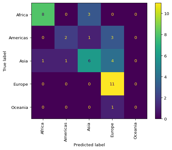
The confusion matrix helps diagnose model performance. If certain classes are frequently confused with each other, this might suggest that those classes are genuinely similar according to the available predictors, or that additional predictors are needed to distinguish them.
Rather than just predicting the most likely class, classification models can provide the probability of each class. These probabilities are useful for understanding model confidence and for applications where the costs of different types of errors vary.
model.predict_proba()
shape: (135, 9)
| index_ | target_ | prediction_ | prob_pred_ | Africa | Americas | Asia | Europe | Oceania |
|---|---|---|---|---|---|---|---|---|
| str | str | str | f64 | f64 | f64 | f64 | f64 | f64 |
| "test" | "Africa" | "Africa" | 0.759861 | 0.759861 | 0.05542 | 0.166569 | 0.013719 | 0.004431 |
| "test" | "Americas" | "Asia" | 0.342032 | 0.267805 | 0.270034 | 0.342032 | 0.106992 | 0.013136 |
| "test" | "Europe" | "Europe" | 0.636839 | 0.00973 | 0.23423 | 0.110382 | 0.636839 | 0.00882 |
| "test" | "Americas" | "Europe" | 0.757296 | 0.009671 | 0.03303 | 0.192822 | 0.757296 | 0.007181 |
| "train" | "Asia" | "Asia" | 0.548589 | 0.182781 | 0.038866 | 0.548589 | 0.212987 | 0.016778 |
| … | … | … | … | … | … | … | … | … |
| "train" | "Europe" | "Asia" | 0.442416 | 0.102468 | 0.16901 | 0.442416 | 0.270195 | 0.01591 |
| "train" | "Asia" | "Europe" | 0.400506 | 0.092076 | 0.156948 | 0.334115 | 0.400506 | 0.016356 |
| "test" | "Americas" | "Americas" | 0.398278 | 0.307302 | 0.398278 | 0.200639 | 0.082725 | 0.011056 |
| "train" | "Asia" | "Europe" | 0.674075 | 0.021438 | 0.071544 | 0.221415 | 0.674075 | 0.011529 |
| "test" | "Asia" | "Africa" | 0.724344 | 0.724344 | 0.035139 | 0.219583 | 0.01615 | 0.004784 |
The output includes the predicted class, the maximum probability (the confidence in that prediction), and the probability assigned to each possible class. Observations with high maximum probability are those where the model is most confident; observations with probabilities spread across multiple classes are more uncertain.
For multinomial classification, there are separate coefficients for each class. Each set of coefficients describes how the predictors relate to the probability of that particular class relative to the others.
model.coef()
shape: (5, 6)
| name | Africa | Americas | Asia | Europe | Oceania |
|---|---|---|---|---|---|
| str | f64 | f64 | f64 | f64 | f64 |
| "Intercept" | 0.408163 | 0.099448 | 1.175146 | 0.484351 | -2.167108 |
| "hdi" | -1.786831 | 0.0 | 0.0 | 0.758943 | 0.0 |
| "gdp" | 0.0 | -0.770247 | 0.0 | 0.500606 | 0.0 |
| "cellphone" | 0.0 | 0.0 | -0.407828 | 0.0 | 0.0 |
| "happy" | -0.078951 | 1.039058 | -0.038636 | 0.0 | 0.0 |
Interpreting these coefficients is more complex than in binary logistic regression. A positive coefficient for a predictor in a particular class means that higher values of that predictor are associated with higher probability of that class, all else being equal. However, because the probabilities must sum to one, the effects are relative rather than absolute.
Gradient boosting can also be applied to classification problems. The algorithm adapts to predict class probabilities rather than numeric values, using a suitable loss function for classification.
model = (
    country
    .pipe(
        DSSklearn.gradient_boosting_classifier,
        target=c.region,
        features=[c.hdi, c.gdp, c.cellphone, c.happy],
        n_estimators=100,
        learning_rate=0.1,
        max_depth=3
    )
)model.score(){'train': 1.0, 'test': 0.5609756097560976}Gradient boosting classifiers can capture complex, nonlinear relationships between predictors and class membership. However, they can also overfit, especially with small datasets or many trees. A common sign of overfitting is a large gap between training accuracy (often very high) and testing accuracy.
model.predict_proba()
shape: (135, 9)
| index_ | target_ | prediction_ | prob_pred_ | Africa | Americas | Asia | Europe | Oceania |
|---|---|---|---|---|---|---|---|---|
| str | str | str | f64 | f64 | f64 | f64 | f64 | f64 |
| "train" | "Africa" | "Africa" | 0.997384 | 0.997384 | 0.000019 | 0.002568 | 0.00003 | 6.4561e-8 |
| "train" | "Americas" | "Americas" | 0.989996 | 0.000388 | 0.989996 | 0.009259 | 0.000356 | 0.000001 |
| "test" | "Europe" | "Europe" | 0.87997 | 0.000325 | 0.00182 | 0.11783 | 0.87997 | 0.000055 |
| "train" | "Americas" | "Americas" | 0.987193 | 0.000428 | 0.987193 | 0.003594 | 0.008783 | 0.000002 |
| "train" | "Asia" | "Asia" | 0.988641 | 0.006167 | 0.002201 | 0.988641 | 0.002984 | 0.000007 |
| … | … | … | … | … | … | … | … | … |
| "train" | "Europe" | "Europe" | 0.989236 | 0.001594 | 0.000423 | 0.008745 | 0.989236 | 0.000002 |
| "test" | "Asia" | "Americas" | 0.924516 | 0.003275 | 0.924516 | 0.031698 | 0.040502 | 0.00001 |
| "train" | "Americas" | "Americas" | 0.997708 | 0.000027 | 0.997708 | 0.002261 | 0.000004 | 8.0347e-8 |
| "train" | "Asia" | "Asia" | 0.982414 | 0.000115 | 0.001206 | 0.982414 | 0.016265 | 3.4410e-7 |
| "train" | "Asia" | "Asia" | 0.978957 | 0.016793 | 0.001649 | 0.978957 | 0.002596 | 0.000006 |
Notice that gradient boosting often produces very confident predictions — probabilities close to 0 or 1 — even when accuracy is moderate. This overconfidence can be problematic in applications where calibrated probability estimates are important. The learning rate and number of trees can be adjusted to reduce overfitting, though this may also reduce accuracy.
Choosing Between Methods
The choice between logistic regression and gradient boosting (or other methods) depends on the specific problem. Logistic regression is simpler, more interpretable, and often works well when relationships between predictors and class membership are approximately linear. Gradient boosting is more flexible and can capture complex patterns, but is harder to interpret and more prone to overfitting. In practice, it is common to try multiple methods and compare their performance on testing data.
11.9 Conclusion
This chapter introduced the fundamental concepts of supervised learning, the branch of machine learning focused on making predictions from data. We began by distinguishing predictive modeling from statistical inference: while both involve modeling relationships in data, inference emphasizes understanding and testing those relationships, while prediction emphasizes accurate forecasting for new observations.
The central challenge in predictive modeling is overfitting — fitting the training data so closely that the model fails to generalize to new data. We addressed this challenge through the train-test split, which evaluates models on data not used in training, and through regularization techniques like the lasso and ridge regression, which penalize complex models to improve generalization.
We explored several modeling approaches. Linear regression, familiar from the previous chapter, provides a baseline for regression problems. Regularization methods improve upon basic linear regression by preventing overfitting and, in the case of the lasso, performing variable selection. Gradient boosting offers a powerful alternative that can capture nonlinear relationships, at the cost of interpretability.
For classification problems, we extended logistic regression to multiple classes and applied similar regularization techniques. Gradient boosting classifiers provide a flexible alternative, though they require careful tuning to avoid overconfidence in predictions.
Throughout, we emphasized the importance of proper evaluation. Training error measures how well a model fits known data; testing error measures how well it predicts new data. Models should be selected and tuned based on testing performance, not training performance. This principle — never trust a model’s performance on the same data used to build it — is perhaps the most important lesson of supervised learning.
The techniques introduced here form the foundation for more advanced methods we will explore in subsequent chapters. Deep learning extends these ideas with more flexible model architectures, while careful feature engineering and model selection can further improve predictions. Regardless of the specific method used, the core principles remain the same: learn patterns from labeled data, evaluate on held-out data, and guard against overfitting.