import numpy as np
import polars as pl

from funs import *
from plotnine import *
from polars import col as c
theme_set(theme_minimal())

import spacy

meta = pl.read_csv("data/wiki_uk_meta.csv.gz")
docs = pl.read_csv("data/wiki_uk_authors_text.csv")
docs_fr = pl.read_csv("data/wiki_uk_authors_text_fr.csv")19 Textual Data
19.1 Setup
Load all of the modules and datasets needed for the chapter. We also load the spacy module designed specifically for processing large collections of text.
19.2 Introduction
Every dataset we have encountered so far in this book has consisted of structured observations: rows with well-defined columns containing numbers, categories, or dates. But an enormous amount of the world’s information exists as unstructured text. Medical records contain free-text physician notes alongside coded diagnoses. Customer feedback arrives as open-ended survey responses. Historical archives preserve centuries of human thought in letters, newspapers, and books. Social scientists study political speeches, journalists analyze leaked documents, and humanists trace the evolution of literary style across generations.
Working with textual data requires a fundamentally different approach than working with numbers. A sentence is not just a sequence of characters but a structured object with grammar, meaning, and context. The word “bank” means something different in “river bank” than in “bank account.” The phrase “not bad” typically means something positive despite containing a negation. These subtleties make text both rich and challenging to analyze computationally.
In this chapter, we introduce tools for transforming unstructured text into structured data that can be analyzed using the techniques developed throughout this book. The key insight is that once we have converted text into tables of tokens, counts, and annotations, we can apply familiar operations like filtering, grouping, and joining to answer questions about language. What words distinguish one author from another? Which terms best summarize a document? How does writing style vary across languages or time periods?
We will use spaCy, a modern natural language processing library, to handle the linguistic heavy lifting. SpaCy provides pre-trained models that can tokenize text, identify parts of speech, recognize named entities, and parse grammatical structure. Our job is to take the output of these models and reshape it into forms suitable for analysis.
19.3 NLP Pipeline
We load spaCy’s English language model, which contains statistical models trained on large corpora of English text. The “sm” suffix indicates the small model, which balances accuracy with speed and memory usage. Larger models are available for applications requiring higher precision.
nlp = spacy.load("en_core_web_sm")Our primary dataset consists of Wikipedia pages for authors from the United Kingdom. We have a metadata table containing information about each author.
meta
shape: (75, 7)
| doc_id | born | died | era | gender | link | short |
|---|---|---|---|---|---|---|
| str | i64 | i64 | str | str | str | str |
| "Marie de France" | 1160 | 1215 | "Early" | "female" | "Marie_de_France" | "Marie d. F." |
| "Geoffrey Chaucer" | 1343 | 1400 | "Early" | "male" | "Geoffrey_Chaucer" | "Chaucer" |
| "John Gower" | 1330 | 1408 | "Early" | "male" | "John_Gower" | "Gower" |
| "William Langland" | 1332 | 1386 | "Early" | "male" | "William_Langland" | "Langland" |
| "Margery Kempe" | 1373 | 1438 | "Early" | "female" | "Margery_Kempe" | "Kempe" |
| … | … | … | … | … | … | … |
| "Stephen Spender" | 1909 | 1995 | "Twentieth C" | "male" | "Stephen_Spender" | "Spender" |
| "Christopher Isherwood" | 1904 | 1986 | "Twentieth C" | "male" | "Christopher_Isherwood" | "Isherwood" |
| "Edward Upward" | 1903 | 2009 | "Twentieth C" | "male" | "Edward_Upward" | "Upward" |
| "Rex Warner" | 1905 | 1986 | "Twentieth C" | "male" | "Rex_Warner" | "Warner" |
| "Seamus Heaney" | 1939 | 1939 | "Twentieth C" | "male" | "Seamus_Heaney" | "Heaney" |
As well as a seperate file giving each of the texts from the documents.
docs
shape: (75, 2)
| doc_id | text |
|---|---|
| str | str |
| "Marie de France" | "Marie de France was a poet pos… |
| "Geoffrey Chaucer" | "Geoffrey Chaucer was an Englis… |
| "John Gower" | "John Gower was an English poet… |
| "William Langland" | "William Langland is the presum… |
| "Margery Kempe" | "Margery Kempe was an English C… |
| … | … |
| "Stephen Spender" | "Sir Stephen Harold Spender CBE… |
| "Christopher Isherwood" | "Christopher William Bradshaw I… |
| "Edward Upward" | "Edward Falaise Upward FRSL was… |
| "Rex Warner" | "Rex Warner was an English clas… |
| "Seamus Heaney" | "Seamus Justin Heaney MRIA was … |
The metadata table contains structured information extracted from Wikipedia’s infoboxes: birth and death dates, occupations, and other biographical details. The text table contains the prose content of each page, which we will process using natural language techniques.
Natural language processing transforms raw text into structured annotations. The DSText.process method sends each document through spaCy’s processing pipeline, which performs several analyses in sequence: tokenization (splitting text into words and punctuation), part-of-speech tagging (identifying nouns, verbs, adjectives), lemmatization (reducing words to their base forms), named entity recognition (identifying people, places, organizations), and dependency parsing (analyzing grammatical relationships).
anno = DSText.process(docs, nlp)
anno
shape: (408_700, 15)
| doc_id | sid | tid | token | token_with_ws | lemma | upos | tag | is_alpha | is_stop | is_punct | dep | head_idx | ent_type | ent_iob |
|---|---|---|---|---|---|---|---|---|---|---|---|---|---|---|
| str | i64 | i64 | str | str | str | str | str | bool | bool | bool | str | i64 | str | str |
| "Marie de France" | 1 | 1 | "Marie" | "Marie " | "Marie" | "PROPN" | "NNP" | true | false | false | "compound" | 3 | "PERSON" | "B" |
| "Marie de France" | 1 | 2 | "de" | "de " | "de" | "X" | "FW" | true | false | false | "nmod" | 3 | "PERSON" | "I" |
| "Marie de France" | 1 | 3 | "France" | "France " | "France" | "PROPN" | "NNP" | true | false | false | "nsubj" | 4 | "PERSON" | "I" |
| "Marie de France" | 1 | 4 | "was" | "was " | "be" | "AUX" | "VBD" | true | true | false | "ROOT" | 4 | "" | "O" |
| "Marie de France" | 1 | 5 | "a" | "a " | "a" | "DET" | "DT" | true | true | false | "det" | 6 | "" | "O" |
| … | … | … | … | … | … | … | … | … | … | … | … | … | … | … |
| "Seamus Heaney" | 242 | 18 | "of" | "of " | "of" | "ADP" | "IN" | true | true | false | "prep" | 17 | "" | "O" |
| "Seamus Heaney" | 242 | 19 | "his" | "his " | "his" | "PRON" | "PRP$" | true | true | false | "poss" | 21 | "" | "O" |
| "Seamus Heaney" | 242 | 20 | "finest" | "finest " | "fine" | "ADJ" | "JJS" | true | false | false | "amod" | 21 | "" | "O" |
| "Seamus Heaney" | 242 | 21 | "poems" | "poems" | "poem" | "NOUN" | "NNS" | true | false | false | "pobj" | 18 | "" | "O" |
| "Seamus Heaney" | 242 | 22 | "." | "." | "." | "PUNCT" | "." | false | false | true | "punct" | 8 | "" | "O" |
There is a lot of information that has been automatically added to this table, thanks to the collective results of decades of research in computational linguistics and natural language processing. Each row corresponds to a word or a punctuation mark (created by the process of tokenization), along with metadata describing the token. Notice that reading down the column token reproduces the original text. The columns available are:
- doc_id: A key that allows us to group tokens into documents and to link back into the original input table.
- sid: Numeric identifier of the sentence number.
- tid: Numeric identifier of the token within a sentence. The first three columns form a primary key for the table.
- token: A character variable containing the detected token, which is either a word or a punctuation mark.
- token_with_ws: The token with white space (spaces and new-line characters) added. This is useful if we wanted to re-create the original text from the token table.
- lemma: A normalized version of the token. For example, it removes start-of-sentence capitalization, turns all nouns into their singular form, and converts verbs into their infinitive form.
- upos: The universal part of speech code, which are parts of speech that can be defined in most spoken languages. These tend to correspond to the parts of speech taught in primary schools, such as “NOUN”, “ADJ” (adjective), and “ADV” (adverb).
- tag: A fine-grained part of speech code that depends on the specific language (here, English) and models being used.
- is_alpha, is_stop, is_punct: Boolean flags for alphabetic characters, stop words, and punctuation.
- dep: The dependency relation label describing how this token relates grammatically to another token.
- head_idx: The token index of the word in the sentence that this token is grammatically related to.
- ent_type: The named entity type, if this token is part of a recognized entity.
There are many analyses that can be performed on the extracted features that are present in the anno table. Fortunately, many of these can be performed by directly using Polars operations covered in the first five chapters of this text, without the need for any new text-specific functions. For example, we can find the most common nouns in the dataset by filtering on the universal part of speech and grouping by lemma with the code below.
(
    anno
    .filter(c.upos == "NOUN")
    .group_by(c.lemma)
    .agg(count = pl.len())
    .sort(c.count, descending=True)
    .head(10)
)
shape: (10, 2)
| lemma | count |
|---|---|
| str | u32 |
| "work" | 1154 |
| "year" | 1012 |
| "time" | 846 |
| "poem" | 744 |
| "life" | 740 |
| "book" | 591 |
| "death" | 540 |
| "novel" | 527 |
| "poet" | 513 |
| "family" | 467 |
The most frequent nouns across the set of documents roughly fall into one of two categories. Those such as “year”, “life”, “death”, and “family” are nouns that we would frequently associate with biographical entries for nearly any group of people. Others, such as “poem”, “book”, “poet”, and the somewhat more generic “work”, capture the specific objects that authors would produce and therefore would be prominent elements of their respective Wikipedia pages. The fact that these two types of nouns show up at the top of the list helps to verify that both the dataset and the NLP pipeline are working as expected.
We can use a similar technique to learn about the contents of each of the individual documents. Suppose we wanted to know which adjectives are most used on each page. This can be done by a sequence of Polars operations. First, we filter the data by the part of speech and group the rows of the dataset by the document id and lemma. Then, we count the number of rows for each unique combination of document and lemma and arrange the dataset in descending order of count. We can use the head() method on grouped data to take the most frequent adjectives within each document:
(
    anno
    .filter(c.upos == "ADJ")
    .group_by([c.doc_id, c.lemma])
    .agg(count = pl.len())
    .sort([c.doc_id, c.count], descending=[False, True])
    .group_by(c.doc_id)
    .head(8)
    .group_by(c.doc_id)
    .agg(top_adj = c.lemma.sort().str.join("; "))
)
shape: (75, 2)
| doc_id | top_adj |
|---|---|
| str | str |
| "Virginia Woolf" | "first; literary; many; much; o… |
| "A. A. Milne" | "british; considerable; many; m… |
| "James Joyce" | "british; english; first; irish… |
| "Matthew Arnold" | "first; good; great; literary; … |
| "Katherine Philipps" | "cavalier; female; french; lite… |
| … | … |
| "W. H. Auden" | "american; first; late; later; … |
| "Charlotte Smith" | "first; legal; literary; many; … |
| "George Orwell" | "-; english; first; good; liter… |
| "John Stuart Mill" | "great; high; more; other; own;… |
| "John Gower" | "early; english; first; much; o… |
The output shows many connections between adjectives and the authors. Here, the connections again fall roughly into two groups. Some of the adjectives are fairly generic—such as “more”, “other”, and “many”—and probably say more about the people writing the pages than the subjects of the pages themselves. Other adjectives provide more contextual information about each of the authors. For example, several selected adjectives are key descriptions of an author’s work, such as “Victorian” associated with certain authors and “Gothic” with others. While it is good to see expected relationships to demonstrate the data and techniques are functioning properly, it is also valuable when computational techniques highlight the unexpected.
19.4 N-grams and Collocations
So far we have analyzed individual words in isolation. But meaning often emerges from combinations of words. The phrase “New York” refers to a specific city, not something novel and a name. “Machine learning” describes a field of study, not appliances that acquire knowledge. “Poet laureate” is a title, not just any poet who happens to be a laureate. To capture these multi-word expressions, we turn to n-grams: contiguous sequences of n tokens.
A unigram is a single token (what we have been working with). A bigram is a pair of adjacent tokens. A trigram is a sequence of three tokens. In general, an n-gram captures local word order, which is lost when we treat documents as unordered collections of words.
Constructing n-grams requires us to look at tokens in context. Polars window functions allow us to access neighboring rows, which we can use to pair each token with the tokens that follow it. The key is to shift the token column to align adjacent words on the same row.
bigrams = (
    anno
    .filter(c.is_alpha)
    .with_columns(
        next_token = c.lemma.shift(-1).over([c.doc_id, c.sid]),
        next_is_alpha = c.is_alpha.shift(-1).over([c.doc_id, c.sid])
    )
    .filter(c.next_is_alpha == True)
    .with_columns(
        bigram = c.lemma + " " + c.next_token
    )
)
bigrams.select(c.doc_id, c.sid, c.tid, c.lemma, c.next_token, c.bigram)
shape: (363_449, 6)
| doc_id | sid | tid | lemma | next_token | bigram |
|---|---|---|---|---|---|
| str | i64 | i64 | str | str | str |
| "Marie de France" | 1 | 1 | "Marie" | "de" | "Marie de" |
| "Marie de France" | 1 | 2 | "de" | "France" | "de France" |
| "Marie de France" | 1 | 3 | "France" | "be" | "France be" |
| "Marie de France" | 1 | 4 | "be" | "a" | "be a" |
| "Marie de France" | 1 | 5 | "a" | "poet" | "a poet" |
| … | … | … | … | … | … |
| "Seamus Heaney" | 242 | 16 | "inspire" | "many" | "inspire many" |
| "Seamus Heaney" | 242 | 17 | "many" | "of" | "many of" |
| "Seamus Heaney" | 242 | 18 | "of" | "his" | "of his" |
| "Seamus Heaney" | 242 | 19 | "his" | "fine" | "his fine" |
| "Seamus Heaney" | 242 | 20 | "fine" | "poem" | "fine poem" |
The shift(-1) operation moves each column up by one position within each document and sentence, so that each row contains both the current token and the following token. We filter to keep only cases where both tokens are alphabetic, excluding bigrams that span punctuation or sentence boundaries.
Now we can count bigram frequencies just as we counted unigram frequencies:
(
    bigrams
    .group_by(c.bigram)
    .agg(count = pl.len())
    .sort(c.count, descending=True)
    .head(15)
)
shape: (15, 2)
| bigram | count |
|---|---|
| str | u32 |
| "of the" | 3254 |
| "in the" | 2374 |
| "to the" | 1138 |
| "of his" | 1009 |
| "he be" | 963 |
| … | … |
| "on the" | 691 |
| "it be" | 654 |
| "for the" | 647 |
| "in his" | 628 |
| "be the" | 611 |
The most frequent bigrams by raw counts largely consist of functional phrases that appear in many types of text. The phrase “of the” appears often simply because both words are common, not because they form a meaningful unit. To identify true collocations—word pairs that occur together more often than chance would predict—we use pointwise mutual information (PMI). PMI compares the observed frequency of a bigram to the frequency we would expect if the two words were independent:
\[ \text{PMI}(w_1, w_2) = \log_2 \frac{P(w_1, w_2)}{P(w_1) \cdot P(w_2)} \]
A high PMI indicates that the words co-occur much more frequently than their individual frequencies would suggest. A PMI of zero means the words are independent. Negative PMI (rare in practice for bigrams that actually occur) would indicate the words avoid each other.
To compute this we need a few intermediate steps. First of all, we can count the number of times each word appears in all of the texts.
word_counts = (
    anno
    .filter(c.is_alpha)
    .group_by(c.lemma)
    .agg(word_count = pl.len())
)

total_words = anno.filter(c.is_alpha).height
Then, we could the number of teachings each bigram occurs.
bigram_counts = (
    bigrams
    .group_by(c.bigram, c.lemma, c.next_token)
    .agg(bigram_count = pl.len())
)

total_bigrams = bigrams.height
And, finally, we can combine the data together to get the PMI scores for each bigram and sort to find those with the highest scores.
(
    bigram_counts
    .join(
        word_counts.rename({"lemma": "w1", "word_count": "w1_count"}),
        left_on="lemma",
        right_on="w1"
    )
    .join(
        word_counts.rename({"lemma": "w2", "word_count": "w2_count"}),
        left_on="next_token",
        right_on="w2"
    )
    .with_columns(
        p_bigram = c.bigram_count / total_bigrams,
        p_w1 = c.w1_count / total_words,
        p_w2 = c.w2_count / total_words
    )
    .with_columns(
        pmi = (c.p_bigram / (c.p_w1 * c.p_w2)).log() / np.log(2)
    )
    .filter(c.bigram_count >= 5)
    .sort(c.pmi, descending=True)
    .select(c.bigram, c.bigram_count, c.pmi)
    .head(15)
)
shape: (15, 3)
| bigram | bigram_count | pmi |
|---|---|---|
| str | u32 | f64 |
| "El Dorado" | 5 | 16.27981 |
| "Lang Syne" | 5 | 16.27981 |
| "Corpus Christi" | 5 | 16.016776 |
| "magnum opus" | 5 | 16.016776 |
| "Biographia Literaria" | 6 | 16.016776 |
| … | … | … |
| "Luis Borges" | 6 | 15.794384 |
| "gross indecency" | 5 | 15.794384 |
| "Encyclopædia Britannica" | 7 | 15.794384 |
| "MolotovRibbentrop Pact" | 6 | 15.794384 |
| "Vox Clamantis" | 5 | 15.794384 |
The high-PMI bigrams tell a different story than the high-frequency bigrams. These are phrases where the component words strongly predict each other: proper names, technical terms, and domain-specific expressions. Many of these would be good candidates for treating as single units in downstream analysis.
We can extend the same logic to trigrams by shifting twice:
(
    anno
    .filter(c.is_alpha)
    .with_columns(
        next_token = c.lemma.shift(-1).over([c.doc_id, c.sid]),
        next_next_token = c.lemma.shift(-2).over([c.doc_id, c.sid]),
        next_is_alpha = c.is_alpha.shift(-1).over([c.doc_id, c.sid]),
        next_next_is_alpha = c.is_alpha.shift(-2).over([c.doc_id, c.sid])
    )
    .filter((c.next_is_alpha == True) & (c.next_next_is_alpha == True))
    .with_columns(
        trigram = c.lemma + " " + c.next_token + " " + c.next_next_token
    )
    .group_by(c.trigram)
    .agg(count = pl.len())
    .sort(c.count, descending=True)
    .head(15)
)
shape: (15, 2)
| trigram | count |
|---|---|
| str | u32 |
| "one of the" | 217 |
| "as well as" | 125 |
| "at the time" | 122 |
| "the age of" | 120 |
| "be publish in" | 115 |
| … | … |
| "that he be" | 74 |
| "a number of" | 74 |
| "to have be" | 64 |
| "member of the" | 64 |
| "a series of" | 64 |
Trigrams capture even longer expressions, but again we see the raw scores simply find combinations of frequent words. Extending the code for PMI would be required to get more useful information from this table.
19.5 Named Entity Recognition
Named entity recognition (NER) identifies and classifies proper nouns and other specific references in text. SpaCy’s NER model recognizes several entity types: people (PERSON), organizations (ORG), geopolitical entities like countries and cities (GPE), dates (DATE), works of art (WORK_OF_ART), and others. These annotations are stored in the ent_type column of our token table.
(
    anno
    .filter(c.ent_type != "")
    .select(c.doc_id, c.sid, c.tid, c.token, c.ent_type)
)
shape: (73_326, 5)
| doc_id | sid | tid | token | ent_type |
|---|---|---|---|---|
| str | i64 | i64 | str | str |
| "Marie de France" | 1 | 1 | "Marie" | "PERSON" |
| "Marie de France" | 1 | 2 | "de" | "PERSON" |
| "Marie de France" | 1 | 3 | "France" | "PERSON" |
| "Marie de France" | 1 | 13 | "France" | "GPE" |
| "Marie de France" | 1 | 17 | "England" | "GPE" |
| … | … | … | … | … |
| "Seamus Heaney" | 240 | 17 | "BBC" | "ORG" |
| "Seamus Heaney" | 240 | 18 | "Two" | "CARDINAL" |
| "Seamus Heaney" | 241 | 3 | "Marie" | "PERSON" |
| "Seamus Heaney" | 242 | 3 | "first" | "ORDINAL" |
| "Seamus Heaney" | 242 | 6 | "four" | "CARDINAL" |
Each token that is part of a named entity receives a type label. Multi-word entities like “United Kingdom” have the same label on each constituent token. To work with complete entities rather than individual tokens, we need to group consecutive tokens with the same entity type.
We can identify entity boundaries by detecting where the entity type changes:
entities = (
    anno
    .filter(c.ent_type != "")
    .with_columns(
        new_entity = c.ent_iob == "B"
    )
    .with_columns(
        entity_id = c.new_entity.cum_sum().over([c.doc_id])
    )
    .group_by([c.doc_id, c.entity_id, c.ent_type])
    .agg(
        entity_text = c.token.str.join(" "),
    )
)
entities.select(c.doc_id, c.ent_type, c.entity_text)
shape: (42_261, 3)
| doc_id | ent_type | entity_text |
|---|---|---|
| str | str | str |
| "John Milton" | "NORP" | "English" |
| "John Keats" | "ORDINAL" | "first" |
| "Virginia Woolf" | "GPE" | "Woolfs" |
| "Beatrix Potter" | "ORG" | "Herdwick" |
| "Thomas Malory" | "PERSON" | "Robert Corbet" |
| … | … | … |
| "Oscar Wilde" | "PERSON" | "Henry James" |
| "George Orwell" | "PERSON" | "Stalin" |
| "Charlotte Smith" | "DATE" | "17911793" |
| "Lord Byron" | "FAC" | "the Battle of Alvøen" |
| "Louis MacNeice" | "ORG" | "Merton College Oxford" |
Now we can analyze entities at the appropriate level of granularity. For example, we can find the most frequently mentioned people across all documents:
(
    entities
    .filter(c.ent_type == "PERSON")
    .group_by(c.entity_text)
    .agg(count = pl.len())
    .sort(c.count, descending=True)
    .head(15)
)
shape: (15, 2)
| entity_text | count |
|---|---|
| str | u32 |
| "Johnson" | 239 |
| "Shakespeare" | 183 |
| "Dickens" | 166 |
| "Shelley" | 137 |
| "Joyce" | 136 |
| … | … |
| "Austen" | 81 |
| "Mill" | 80 |
| "Marlowe" | 74 |
| "Lawrence" | 72 |
| "Mary" | 70 |
The most frequently mentioned people likely include both the subjects of the Wikipedia pages and other figures who appear across multiple biographies—editors, patrons, family members, or influential contemporaries.
We can examine which entity types are most common overall:
(
    entities
    .group_by(c.ent_type)
    .agg(count = pl.len())
    .sort(c.count, descending=True)
)
shape: (18, 2)
| ent_type | count |
|---|---|
| str | u32 |
| "PERSON" | 13547 |
| "ORG" | 7412 |
| "DATE" | 7054 |
| "GPE" | 4547 |
| "NORP" | 2864 |
| … | … |
| "TIME" | 143 |
| "LAW" | 77 |
| "QUANTITY" | 73 |
| "MONEY" | 17 |
| "PERCENT" | 1 |
Biographical articles naturally contain many dates (birth, death, publication) and references to people and places. The distribution of entity types provides a high-level characterization of the content.
Entity co-occurrence within documents can reveal relationships. Which people are mentioned together? Which places are associated with which organizations?
# Find all pairs of people mentioned in the same document
people = (
    entities
    .filter(c.ent_type == "PERSON")
    .select(c.doc_id, person = c.entity_text)
)

person_pairs = (
    people
    .join(people, on="doc_id", suffix="_2")
    .filter(c.person < c.person_2)  # Avoid duplicates and self-pairs
    .group_by([c.person, c.person_2])
    .agg(co_occurrences = pl.len())
    .sort(c.co_occurrences, descending=True)
    .head(10)
)
person_pairs
shape: (10, 3)
| person | person_2 | co_occurrences |
|---|---|---|
| str | str | u32 |
| "Mary" | "Shelley" | 3762 |
| "Shaw" | "Shaws" | 3717 |
| "Shelley" | "Shelleys" | 3509 |
| "Johnson" | "Shakespeare" | 3353 |
| "Austen" | "Austens" | 2765 |
| "Dickens" | "Oliver Twist" | 2754 |
| "Jonson" | "Shakespeare" | 2250 |
| "Keats" | "Keatss" | 2241 |
| "Vanessa" | "Woolf" | 2112 |
| "David Copperfield" | "Dickens" | 2107 |
Pairs of people who frequently appear together across documents may have historical connections: collaborators, rivals, members of the same literary movement, or subjects of comparative study.
19.6 Dependency Parsing
While named entities tell us what is mentioned, dependency parsing tells us how words relate grammatically. Each token in a sentence has a head—another token that it modifies or depends on—and a dependency relation describing the nature of that relationship. The root of the sentence is typically the main verb, and all other tokens connect to it through a tree structure.
The dependency annotations are stored in the dep and head_idx columns. Common dependency relations include:
- nsubj: Nominal subject (the doer of an action)
- dobj / obj: Direct object (the receiver of an action)
- amod: Adjectival modifier
- prep / pobj: Prepositional phrases
- compound: Compound words or phrases
- ROOT: The root of the sentence
Let’s look at a particular example from the Seamus Heaney article.
(
    anno
    .filter(c.doc_id == "Seamus Heaney")
    .filter(c.sid == 1)
    .select(c.tid, c.token, c.upos, c.dep, c.head_idx)
)
shape: (12, 5)
| tid | token | upos | dep | head_idx |
|---|---|---|---|---|
| i64 | str | str | str | i64 |
| 1 | "Seamus" | "PROPN" | "compound" | 4 |
| 2 | "Justin" | "PROPN" | "compound" | 4 |
| 3 | "Heaney" | "PROPN" | "compound" | 4 |
| 4 | "MRIA" | "PROPN" | "nsubj" | 5 |
| 5 | "was" | "AUX" | "ROOT" | 5 |
| … | … | … | … | … |
| 8 | "poet" | "NOUN" | "compound" | 9 |
| 9 | "playwright" | "NOUN" | "attr" | 5 |
| 10 | "and" | "CCONJ" | "cc" | 9 |
| 11 | "translator" | "NOUN" | "conj" | 9 |
| 12 | "." | "PUNCT" | "punct" | 5 |
We can use dependency relations to extract specific grammatical patterns. For example, to find what subjects do what actions, we can look for subject-verb pairs.
verbs = (
    anno
    .filter(c.upos == "VERB")
    .select(
        c.doc_id, c.sid,
        verb_idx = c.tid,
        verb = c.lemma
    )
)

(
    anno
    .filter(c.dep == "nsubj")
    .select(
        c.doc_id, c.sid,
        subject = c.lemma,
        verb_idx = c.head_idx
    )
    .join(verbs, on=[c.doc_id, c.sid, c.verb_idx])
    .group_by([c.subject, c.verb])
    .agg(count = pl.len())
    .sort(c.count, descending=True)
    .head(10)
)
shape: (10, 3)
| subject | verb | count |
|---|---|---|
| str | str | u32 |
| "he" | "write" | 273 |
| "he" | "have" | 131 |
| "he" | "become" | 105 |
| "she" | "write" | 79 |
| "he" | "make" | 61 |
| "he" | "meet" | 60 |
| "he" | "begin" | 56 |
| "he" | "say" | 53 |
| "he" | "return" | 52 |
| "he" | "leave" | 51 |
This reveals the typical actions associated with different subjects in our corpus. We might see that authors “write”, “publish”, and “die”, while works “appear”, “receive”, and “influence”.
We can also extract adjective-noun pairs to see how different concepts are described:
(
    anno
    .filter(c.dep == "amod", c.is_alpha)
    .select(
        c.doc_id, c.sid,
        adjective = c.lemma,
        noun_idx = c.head_idx
    )
    .join(
        anno.filter(c.upos == "NOUN").select(
            c.doc_id, c.sid, noun_idx = c.tid, noun = c.lemma,
        ),
        on=[c.doc_id, c.sid, c.noun_idx]
    )
    .group_by([c.adjective, c.noun])
    .agg(count = pl.len())
    .sort(c.count, descending=True)
    .head(10)
)
shape: (10, 3)
| adjective | noun | count |
|---|---|---|
| str | str | u32 |
| "short" | "story" | 60 |
| "next" | "year" | 50 |
| "same" | "time" | 44 |
| "early" | "work" | 44 |
| "same" | "year" | 42 |
| "close" | "friend" | 41 |
| "english" | "poet" | 38 |
| "major" | "work" | 33 |
| "young" | "man" | 32 |
| "literary" | "critic" | 32 |
The adjective-noun combinations reveal the conceptual vocabulary of the corpus: what kinds of things exist in this textual world, and how are they characterized?
19.7 Keyword in Context (KWIC)
Sometimes we want to see how a specific word is used across the corpus. A concordance or keyword in context (KWIC) display shows each occurrence of a target word along with the words that surround it. This technique, which predates computers, remains invaluable for understanding how language is actually used.
To build a KWIC display, we need to extract a window of tokens around each occurrence of our keyword. This logic is implemented in the DSText.kwic method.
kwic_results = DSText.kwic(anno, "poetry", max_num=15, window=5)
kwic_results
Marie de France:101 exhibit a form of lyrical [poetry] that influenced the way that
Marie de France:101 influenced the way that narrative [poetry] was subsequently composed adding another
Geoffrey Chaucer:2 alternatively the father of English [poetry] .
Geoffrey Chaucer:45 introduced him to medieval Italian [poetry] the forms and stories of
Geoffrey Chaucer:110 nettle in Chaucers garden of [poetry] .
Geoffrey Chaucer:118 The [poetry] of Chaucer along with other
Geoffrey Chaucer:147 the enduring interest in his [poetry] prior to the arrival of
John Gower:55 Gowers [poetry] has had a mixed critical
John Gower:56 as the father of English [poetry] .
Thomas More:22 flute and viol and wrote [poetry] .
Edmund Spenser:6 despite their differing views on [poetry] .
Edmund Spenser:22 place at court through his [poetry] but his next significant publication
Edmund Spenser:38 many pens and pieces of [poetry] into his grave with many
Edmund Spenser:41 one hundred pounds for his [poetry] .
Edmund Spenser:84 scholars have noted that his [poetry] does not rehash tradition but The KWIC display reveals patterns that aggregate statistics miss. We can see the actual phrases in which a word appears, the grammatical constructions it participates in, and the semantic contexts that surround it. Is “poetry” typically the subject of a sentence or the object? What verbs and adjectives accompany it?
19.8 Complexity Metrics
Beyond analyzing content, we can characterize the style of texts using quantitative measures of readability and complexity. These metrics, originally developed to assess the difficulty of reading materials for educational purposes, provide useful descriptive statistics for comparing texts.
For example, sentence length is one of the simplest style measures. Longer sentences tend to be more complex and harder to read.
(
    anno
    .group_by([c.doc_id, c.sid])
    .agg(
        n_tokens = pl.len(),
        n_words = c.is_alpha.sum()
    )
    .group_by(c.doc_id)
    .agg(
        mean_sentence_length = c.n_words.mean(),
        max_sentence_length = c.n_words.max(),
        n_sentences = pl.len()
    )
    .sort(c.mean_sentence_length, descending=True)
    .head(10)
)
shape: (10, 4)
| doc_id | mean_sentence_length | max_sentence_length | n_sentences |
|---|---|---|---|
| str | f64 | u32 | u32 |
| "Thomas Malory" | 28.231214 | 83 | 173 |
| "Mary Wollstonecraft" | 25.902878 | 76 | 278 |
| "Samuel Taylor Coleridge" | 25.831858 | 102 | 226 |
| "W. H. Auden" | 25.502222 | 91 | 225 |
| "Marie de France" | 25.481132 | 71 | 106 |
| "John Stuart Mill" | 25.358065 | 118 | 310 |
| "Ben Jonson" | 25.204724 | 82 | 254 |
| "Katherine Philipps" | 25.137931 | 68 | 58 |
| "Christopher Marlowe" | 25.019802 | 150 | 202 |
| "Geoffrey Chaucer" | 25.018182 | 73 | 220 |
Type-token ratio (TTR) measures vocabulary richness: the number of unique words (types) divided by the total number of words (tokens). A higher TTR indicates more varied vocabulary.
(
    anno
    .filter(c.is_alpha)
    .group_by(c.doc_id)
    .agg(
        n_tokens = pl.len(),
        n_types = c.lemma.n_unique()
    )
    .with_columns(
        ttr = c.n_types / c.n_tokens
    )
    .sort(c.ttr, descending=True)
    .head(10)
)
shape: (10, 4)
| doc_id | n_tokens | n_types | ttr |
|---|---|---|---|
| str | u32 | u32 | f64 |
| "Rex Warner" | 726 | 371 | 0.511019 |
| "Felicia Hemans" | 1473 | 691 | 0.469111 |
| "William Langland" | 908 | 407 | 0.448238 |
| "Cecil Day-Lewis" | 1294 | 559 | 0.431994 |
| "Edward Upward" | 1065 | 458 | 0.430047 |
| "John Gower" | 1439 | 606 | 0.421126 |
| "Stephen Spender" | 1798 | 756 | 0.420467 |
| "Christina Rossetti" | 1909 | 779 | 0.408067 |
| "Philip Sidney" | 1542 | 629 | 0.407912 |
| "Katherine Philipps" | 1458 | 585 | 0.401235 |
TTR is sensitive to document length: longer documents naturally have lower TTR because common words get repeated. For fair comparison across documents of different lengths, we can compute TTR on a fixed-size sample of tokens.
Average word length correlates with vocabulary sophistication. Documents using more polysyllabic, Latinate vocabulary will have higher average word lengths.
(
    anno
    .filter(c.is_alpha)
    .with_columns(
        word_length = c.token.str.len_chars()
    )
    .group_by(c.doc_id)
    .agg(
        mean_word_length = c.word_length.mean()
    )
    .sort(c.mean_word_length, descending=True)
    .head(10)
)
shape: (10, 2)
| doc_id | mean_word_length |
|---|---|
| str | f64 |
| "Mary Wollstonecraft" | 5.123455 |
| "John Milton" | 5.099143 |
| "William Shakespeare" | 5.086957 |
| "Rex Warner" | 5.081267 |
| "Percy Bysshe Shelley" | 5.07918 |
| "John Locke" | 5.051898 |
| "Ann Radcliffe" | 5.04314 |
| "Christopher Marlowe" | 5.034824 |
| "Jane Austen" | 5.021875 |
| "William Langland" | 5.020925 |
Finally, function word ratio measures the proportion of grammatical words (articles, prepositions, pronouns) versus content words (nouns, verbs, adjectives). Different genres and styles have characteristic function word profiles.
content_pos = ["NOUN", "VERB", "ADJ", "ADV"]

(
    anno
    .filter(c.is_alpha)
    .with_columns(
        is_content = c.upos.is_in(content_pos)
    )
    .group_by(c.doc_id)
    .agg(
        n_words = pl.len(),
        n_content = c.is_content.sum()
    )
    .with_columns(
        content_ratio = c.n_content / c.n_words
    )
    .sort(c.content_ratio, descending=True)
    .head(10)
)
shape: (10, 4)
| doc_id | n_words | n_content | content_ratio |
|---|---|---|---|
| str | u32 | u32 | f64 |
| "Margaret Cavendish" | 4737 | 2213 | 0.467173 |
| "John Stuart Mill" | 7861 | 3664 | 0.466098 |
| "Charlotte Smith" | 3543 | 1568 | 0.442563 |
| "Joseph Conrad" | 12546 | 5539 | 0.441495 |
| "John Locke" | 5241 | 2300 | 0.438848 |
| "William Shakespeare" | 6532 | 2812 | 0.430496 |
| "Jane Austen" | 8137 | 3494 | 0.429397 |
| "Alexander Pope" | 3256 | 1397 | 0.429054 |
| "Mary Wollstonecraft" | 7201 | 3068 | 0.426052 |
| "George Bernard Shaw" | 11544 | 4896 | 0.424116 |
19.9 TF-IDF
In the the sections above, we saw that counting the number of times each token or lemma occurs in a document is a useful way of quickly summarizing the content of a document. We can formalize this idea by defining the concept of a term-frequency matrix, often abbreviated TF. The matrix consists of a table of rows and columns where: (1) each row corresponds to a document, (2) each column corresponds to a term, and (3) the entries cound the number of times each document contains each term. An example will help explain this. Consider the four following phrases:
- chop the onion
- chop chop chop the garlic
- sauté the garlic in olive oil
- add the onion and olive oil to the pan
This is what the term-frequency matrix looks like:
| add | and | chop | garlic | in | oil | olive | onion | pan | sauté | the | to | |
|---|---|---|---|---|---|---|---|---|---|---|---|---|
| Doc 1 | 0 | 1 | 1 | 1 | 0 | 0 | 0 | 1 | 0 | 0 | 1 | 0 |
| Doc 2 | 0 | 0 | 3 | 1 | 0 | 0 | 0 | 0 | 0 | 0 | 1 | 0 |
| Doc 3 | 0 | 0 | 0 | 1 | 1 | 1 | 1 | 0 | 0 | 1 | 1 | 0 |
| Doc 4 | 1 | 1 | 0 | 0 | 0 | 1 | 1 | 1 | 1 | 0 | 2 | 1 |
The approach of using raw counts can be improved by using a scaled version of the count metric. The issue with raw counts is that they tend to highlight very common words such as “the”, “have”, and “her”. These can be somewhat avoided by removing a pre-compiled set of known common words—often called stopwords or by doing part of speech filtering. These coarse approaches, however, mostly just move the issue down to a slightly less common set of words that also do not necessarily summarize the contents of each document very well. For example, “publisher” is a frequently used term in many of the documents in the Wikipedia collection due to the subject matter, but that does not mean that it is particularly informative since it occurs in almost every page.
A common alternative technique is to combine information about the frequency of a word within a document with the frequency of the term across the entire collection. We return here to the importance of how we define a document, which will shape our analysis. Metrics of this form are known as term frequency–inverse document frequency scores (TF-IDF). A common version of TF-IDF computes a score for every combination of term and document by multiplying the term frequency by the logarithm of the inverse document frequency. The logarithm is a function that is used to make sure that counts do not grow too fast. For example, a count of about 1000 is only approximately twice as big on the logarithmic scale as a count of 25, in comparison to being 40 times larger on a linear scale. Mathematically, we define this TF-IDF function using the following formula, where tf gives the term frequency and df gives the document frequency:
\[ \text{tfidf} = \text{tf} \times \left(\log\left(\frac{N + 1}{\text{df} + 1}\right) + 1 \right) \]
Here, N is the total number of documents. This score gives a measurement of how important a term is in describing a document in the context of the other documents. If we select words with the highest TF-IDF score for each document, these should give a good measurement of what terms best describe each document uniquely from the rest of the collection. Note that while the scaling functions given above are popular choices, they are not universal. Other papers and software may make different choices with moderate effects on the output results.
For comparison, here is what the corresponding TF-IDF matrix looks like for our small example of four phrases. Notice that while the non-zero numbers change from the TF-IDF example, all of the zeros in the original matrix remain zero here.
| add | and | chop | garlic | in | oil | olive | onion | pan | sauté | the | to | |
|---|---|---|---|---|---|---|---|---|---|---|---|---|
| Doc 1 | 0.00 | 1.46 | 1.46 | 1.16 | 0.00 | 0.00 | 0.00 | 1.46 | 0.00 | 0.00 | 1.00 | 0.00 |
| Doc 2 | 0.00 | 0.00 | 4.39 | 1.16 | 0.00 | 0.00 | 0.00 | 0.00 | 0.00 | 0.00 | 1.00 | 0.00 |
| Doc 3 | 0.00 | 0.00 | 0.00 | 1.16 | 2.32 | 1.46 | 1.46 | 0.00 | 0.00 | 2.32 | 1.00 | 0.00 |
| Doc 4 | 2.32 | 1.46 | 0.00 | 0.00 | 0.00 | 1.46 | 1.46 | 1.46 | 2.32 | 0.00 | 2.00 | 2.32 |
Now that we have a conceptual understanding of TF and TF-IDF matrices, let’s see how to construct them in Python. It’s certainly possible to do this directly with Polars methods, but we also have a wrapper function DSText.compute_tfidf that will produce the values for us directly. Rather than producing the wide matrix directly as described in the small examples above, this function pivots the output into a long format (see Chapter 4 for a review of wider versus long), with one non-zero combination of terms and documents in each row. The options min_df and max_df control the proportion of times that a term can appear in documents before we filter it out as being too rare or too common.
tfidf = DSText.compute_tfidf(anno, min_df=0.01, max_df=1.0)
tfidf
shape: (106_352, 7)
| doc_id | lemma | tf | tf_norm | df_docs | idf | tfidf |
|---|---|---|---|---|---|---|
| str | str | u32 | f64 | u32 | f64 | f64 |
| "George Orwell" | "contrast" | 3 | 0.000184 | 28 | 1.963438 | 0.000361 |
| "Henry Vaughan" | "matriculate" | 1 | 0.000436 | 3 | 3.944439 | 0.001718 |
| "George Bernard Shaw" | "critique" | 1 | 0.000087 | 20 | 2.286211 | 0.000198 |
| "Matthew Arnold" | "meaning" | 1 | 0.000298 | 22 | 2.195239 | 0.000654 |
| "John Keats" | "despite" | 3 | 0.00046 | 50 | 1.398908 | 0.000643 |
| … | … | … | … | … | … | … |
| "George Bernard Shaw" | "people" | 5 | 0.000433 | 52 | 1.360441 | 0.000589 |
| "John Keats" | "sibling" | 1 | 0.000153 | 17 | 2.440362 | 0.000374 |
| "T. S. Eliot" | "emigrate" | 1 | 0.000175 | 6 | 3.384823 | 0.000593 |
| "Charlotte Brontë" | "Patrick" | 5 | 0.001488 | 9 | 3.028148 | 0.004506 |
| "John Stuart Mill" | "housemaid" | 1 | 0.000127 | 3 | 3.944439 | 0.000502 |
Once we have this table, we can combine the top terms from each document to characterize their themes.
(
    tfidf
    .sort([c.doc_id, c.tfidf], descending=[False, True])
    .group_by(c.doc_id)
    .head(10)
    .group_by(c.doc_id)
    .agg(top_lemmas = c.lemma.str.join("; "))
)
shape: (75, 2)
| doc_id | top_lemmas |
|---|---|
| str | str |
| "Oscar Wilde" | "Wilde; the; be; of; and; to; i… |
| "George Herbert" | "the; Herbert; of; in; be; and;… |
| "John Donne" | "Donne; the; of; in; be; Donnes… |
| "Daphne du Maurier" | "Maurier; the; du; be; her; of;… |
| "Louis MacNeice" | "MacNeice; the; and; in; be; of… |
| … | … |
| "Charlotte Smith" | "the; and; Smith; her; of; she;… |
| "George Bernard Shaw" | "the; Shaw; in; and; of; be; a;… |
| "William Wordsworth" | "the; of; Wordsworth; in; and; … |
| "Felicia Hemans" | "the; Hemans; and; of; be; in; … |
| "Samuel Beckett" | "Beckett; the; in; of; and; be;… |
The top TF-IDF terms for each document tend to be proper nouns and domain-specific vocabulary that distinguish one article from another. Compare these to the simple frequency counts from earlier: TF-IDF successfully downweights generic terms like “year” and “work” that appear across all biographies.
19.10 Documents as Vectors
The TF-IDF matrix introduced above contains a row for each document and a column for each term, with the TF-IDF weight in each cell. There is a powerful way to think about this structure: each row of the matrix is a list of numbers that describes a document. We can interpret this list of numbers as a set of coordinates, turning each document into a point in space. This geometric perspective is the key insight that connects textual analysis to the full toolkit of statistical modeling, dimensionality reduction, and prediction that we have developed throughout this book.
To build intuition for this idea, let’s start with just two terms. Suppose we look at the TF-IDF scores for the lemmas “poem” and “novel” across our collection of author pages. Each document has a TF-IDF score for “poem” and a TF-IDF score for “novel”, giving us two numbers per document. We can plot these as coordinates on a standard scatter plot, with one axis for each term.
(
    tfidf
    .filter(c.lemma.is_in(["poem", "novel"]))
    .pivot(on="lemma", index="doc_id", values="tfidf")
    .fill_null(0)
    .pipe(ggplot, aes("poem", "novel"))
    + geom_text(aes(label = "doc_id"), size=7)
)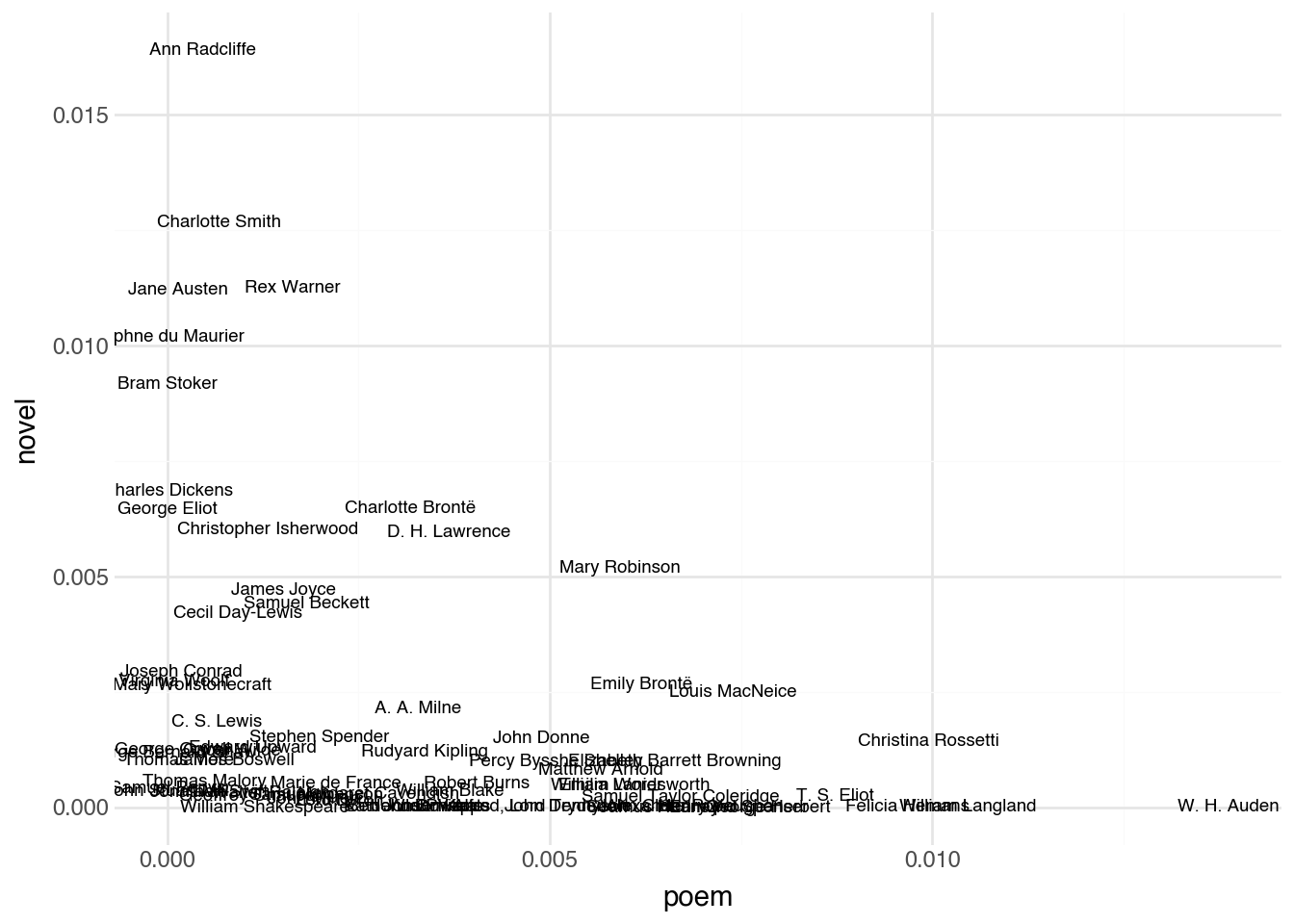
In this two-dimensional view, the position of each document tells us something meaningful. Authors whose Wikipedia pages discuss poetry extensively appear far to the right. Those whose pages focus on novels appear near the top. Authors associated with both forms sit in the upper-right region, while those associated with neither sit near the origin. Documents that are close together in this space have similar usage patterns for these two terms.
Now imagine extending this idea beyond two terms. Rather than plotting documents along axes for just “poem” and “novel”, we could add a third axis for “play”, creating a three-dimensional space where each document is a point. We could keep going: add axes for “war”, “london”, “publish”, “child”, and every other term in our vocabulary. If the vocabulary contains \(V\) terms, each document becomes a point in \(V\)-dimensional space. Mathematically, we represent document \(d\) as a vector of TF-IDF scores:
\[ \mathbf{x}_d = \begin{bmatrix} \text{tfidf}(t_1, d) \\ \text{tfidf}(t_2, d) \\ \vdots \\ \text{tfidf}(t_V, d) \end{bmatrix} \]
We cannot visualize a space with thousands of dimensions, but the geometry works the same way regardless of dimensionality. Two documents that are close together in this high-dimensional space use similar vocabulary in similar proportions. Two documents that are far apart use very different language. The notion of distance between points, which is easy to picture with two terms on a scatter plot, extends naturally to any number of dimensions.
This is a genuinely powerful realization, because once documents are represented as points in a numeric space, every quantitative technique we have encountered in this book becomes available. We can apply dimensionality reduction methods like PCA or UMAP to project the high-dimensional points down to two dimensions for visualization. We can use prediction models to classify documents into categories based on their position in the space. We can run clustering algorithms to discover groups of similar documents automatically. The text has been converted from unstructured prose into a structured numeric representation, and all of the standard tools apply.
One important feature of these document vectors is that most of their entries are zero. Any given document uses only a small fraction of the total vocabulary, so most TF-IDF scores are zero. A vector with mostly zero entries is called sparse, and this representation is sometimes called a sparse embedding. Despite the large number of dimensions, the actual information content of each vector is modest, which matters for computational efficiency but does not change how we think about the geometry.
The code below puts this idea into practice. It constructs a document-term matrix from our annotated text and then applies UMAP to project the high-dimensional document vectors down to two dimensions for visualization. Documents that use similar vocabulary will appear near each other in the resulting plot.
(
    anno
    .pipe(
        DSSklearnText.umap,
        doc_id=c.doc_id,
        term_id=c.lemma,
        n_components=2,
        min_df=0.01,
        max_df=0.5
    )
    .predict(full=True)
    .pipe(ggplot, aes("dr0", "dr1"))
    + geom_text(aes(label = "doc_id"), size=8)
)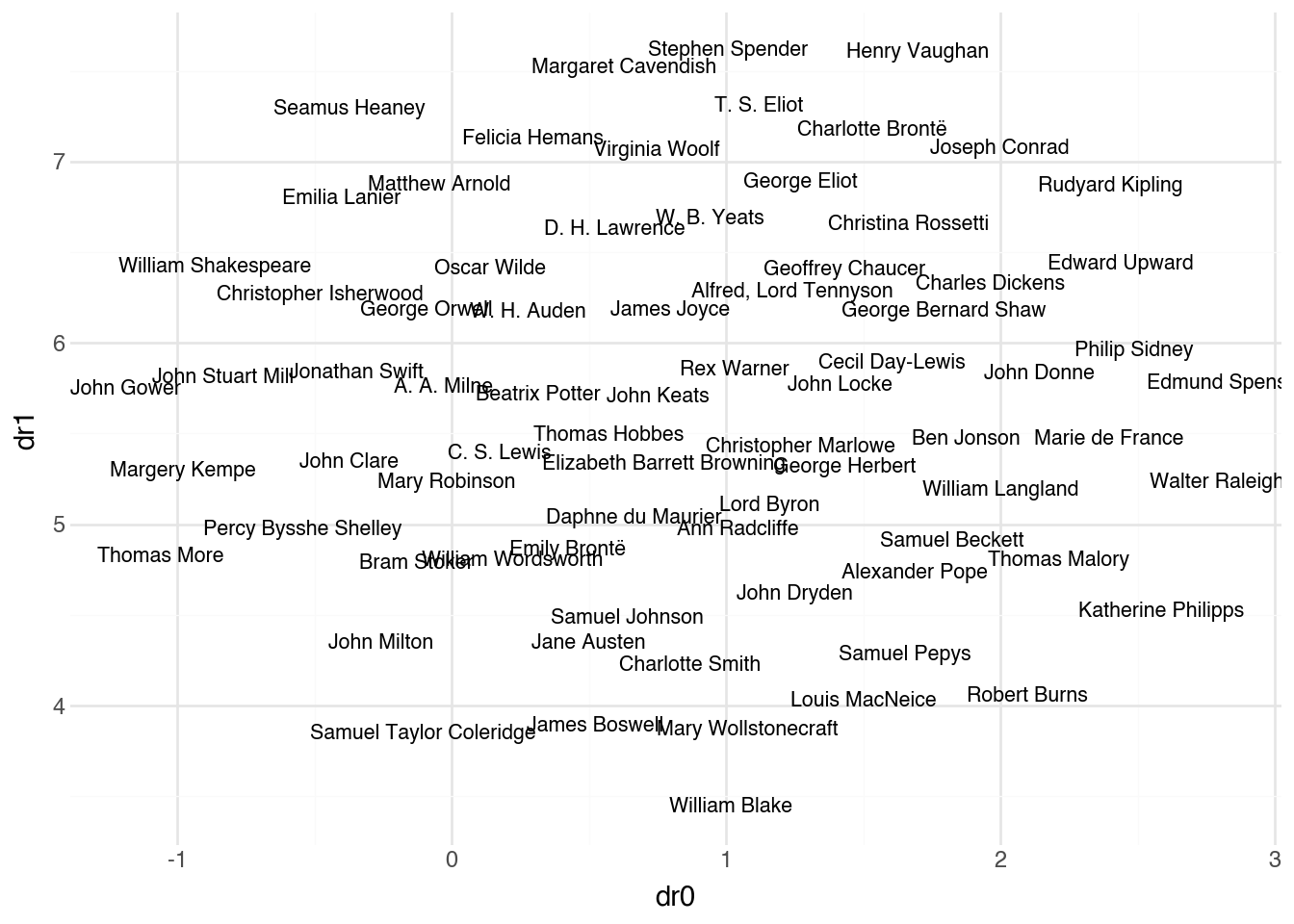
The min_df and max_df parameters filter the vocabulary before constructing the document vectors: terms appearing in fewer than 1% of documents or more than 50% of documents are excluded. This removes both rare terms (which add noise) and ubiquitous terms (which add no discriminative power), focusing the representation on the most informative vocabulary. The UMAP algorithm then finds a two-dimensional arrangement that preserves, as much as possible, the distances between documents in the original high-dimensional space. The result is a map of the corpus where proximity reflects similarity in language use.
19.11 Across Languages
One of the reasons that we enjoy using the content of Wikipedia pages as example datasets for textual analysis is that it is possible to get the page text in a large number of different languages. One of the most interesting aspects of textual analysis is that we can apply our techniques to study how differences across languages and cultures affect the way that knowledge is created and distributed.
Let’s see how our text analysis pipeline can be modified to work with Wikipedia pages from the French version of the site. SpaCy provides models for many different languages:
nlp_fr = spacy.load("fr_core_news_sm")And now, we can annotate the text as follows
anno_fr = DSText.process(docs_fr, nlp_fr)
anno_fr
shape: (203_785, 15)
| doc_id | sid | tid | token | token_with_ws | lemma | upos | tag | is_alpha | is_stop | is_punct | dep | head_idx | ent_type | ent_iob |
|---|---|---|---|---|---|---|---|---|---|---|---|---|---|---|
| str | i64 | i64 | str | str | str | str | str | bool | bool | bool | str | i64 | str | str |
| "Marie de France" | 1 | 1 | "Marie" | "Marie " | "marie" | "NOUN" | "NOUN" | true | false | false | "nsubj" | 6 | "PER" | "B" |
| "Marie de France" | 1 | 2 | "de" | "de " | "de" | "ADP" | "ADP" | true | true | false | "case" | 3 | "PER" | "I" |
| "Marie de France" | 1 | 3 | "France" | "France " | "France" | "PROPN" | "PROPN" | true | false | false | "nmod" | 1 | "PER" | "I" |
| "Marie de France" | 1 | 4 | "est" | "est " | "être" | "AUX" | "AUX" | true | true | false | "cop" | 6 | "" | "O" |
| "Marie de France" | 1 | 5 | "une" | "une " | "un" | "DET" | "DET" | true | true | false | "det" | 6 | "" | "O" |
| … | … | … | … | … | … | … | … | … | … | … | … | … | … | … |
| "Seamus Heaney" | 78 | 5 | "multitude" | "multitude " | "multitude" | "NOUN" | "NOUN" | true | false | false | "obj" | 3 | "" | "O" |
| "Seamus Heaney" | 78 | 6 | "de" | "de " | "de" | "ADP" | "ADP" | true | true | false | "case" | 7 | "" | "O" |
| "Seamus Heaney" | 78 | 7 | "doctorats" | "doctorats " | "doctorat" | "NOUN" | "NOUN" | true | false | false | "nmod" | 5 | "" | "O" |
| "Seamus Heaney" | 78 | 8 | "honoris" | "honoris " | "honoris" | "VERB" | "VERB" | true | false | false | "acl" | 7 | "" | "O" |
| "Seamus Heaney" | 78 | 9 | "causa" | "causa" | "causa" | "NOUN" | "NOUN" | true | false | false | "obj" | 3 | "" | "O" |
French and English have different grammatical structures that will be reflected in part-of-speech frequencies. French uses more determiners (articles), while English may use more auxiliary verbs. These differences are linguistic rather than content-based, but they affect how we should interpret comparative analyses.
Cross-linguistic analysis opens up fascinating questions about how knowledge is organized and transmitted across cultures. The same historical figure may be framed differently depending on the national perspective of the Wikipedia editors. Events that are central to one country’s narrative may be peripheral to another’s. Textual analysis provides the tools to investigate these questions systematically.