import numpy as np
import polars as pl

from funs import *
from plotnine import *
from polars import col as c
theme_set(theme_minimal())

from openai import OpenAI

birds = pl.read_parquet("data/birds10.parquet")15 Transfer Learning
15.1 Setup
Load all of the modules and datasets needed for the chapter. We load the openai module to make requests to the OpenAI API in order to work with state-of-the-art transformer models.
15.2 Transfer Learning
In the previous chapter, we saw how to train neural networks from scratch to recognize patterns in image data. While this approach works well for standardized datasets like MNIST, it has significant limitations when applied to real-world problems. Training a deep neural network requires enormous amounts of labeled data, substantial computational resources, and considerable expertise in tuning hyperparameters. For many practical applications, we simply do not have access to millions of labeled training examples, nor do we have weeks of GPU time to dedicate to training.
Transfer learning offers an elegant solution to this problem. The core insight is that the internal representations learned by a neural network trained on one task often capture general features that are useful for many other tasks. Consider a model trained to classify millions of images into thousands of categories. The early layers of such a model learn to detect basic visual features like edges, textures, and shapes. The middle layers combine these into more complex patterns like eyes, wheels, or leaves. Only the final layers specialize to the specific categories in the original training data. If we want to build a classifier for a new set of categories, we can reuse all but the final layers, benefiting from the rich visual representations the model has already learned.
This approach has become the dominant paradigm in modern machine learning. Rather than training models from scratch, practitioners typically start with a pre-trained model and adapt it to their specific task. This dramatically reduces the amount of data and computation required, often by orders of magnitude. A model that would require millions of training examples when built from scratch might achieve excellent performance with just hundreds or thousands of examples when using transfer learning. The technique is so powerful that it accounts for the vast majority of deep learning applications in production today.
In this chapter, we will explore several forms of transfer learning. We begin with the traditional approach of extracting embeddings from a pre-trained image model and using them as features for a downstream classifier. We then examine zero-shot learning, a more recent development that allows classification without any task-specific training. Finally, we apply these same ideas to text data and briefly discuss how to integrate external AI services through APIs.
15.3 Image Embedding
For this chapter we will use a new dataset of images of different bird species. The predictive model that we want to build should learn how to take an image of a bird and identify which of the ten species in our data the bird comes from. This is a more challenging task than MNIST digit recognition for several reasons: the images are larger and more complex, the subjects appear at different scales and orientations, and the differences between species can be subtle.
birds
shape: (1_555, 5)
| label | filepath | index | vit | siglip |
|---|---|---|---|---|
| str | str | str | list[f64] | list[f64] |
| "canary" | "media/birds10/00000.png" | "test" | [0.017947, -0.0305, … 0.003526] | [-0.00611, -0.042975, … -0.031687] |
| "canary" | "media/birds10/00001.png" | "train" | [0.024804, -0.045255, … -0.007233] | [-0.033767, -0.011978, … -0.020352] |
| "canary" | "media/birds10/00002.png" | "train" | [0.050587, -0.024486, … 0.029895] | [-0.033664, -0.008117, … -0.01725] |
| "canary" | "media/birds10/00003.png" | "train" | [0.047036, -0.038993, … -0.008446] | [-0.010029, -0.018192, … -0.009869] |
| "canary" | "media/birds10/00004.png" | "train" | [0.036349, -0.02734, … -0.018185] | [-0.027327, 0.003568, … -0.033407] |
| … | … | … | … | … |
| "swallow" | "media/birds10/01550.png" | "train" | [-0.022461, -0.025098, … -0.061945] | [-0.022029, -0.008476, … -0.003879] |
| "swallow" | "media/birds10/01551.png" | "train" | [-0.000212, -0.003448, … -0.058042] | [-0.02476, -0.016369, … 0.003875] |
| "swallow" | "media/birds10/01552.png" | "train" | [-0.012531, -0.006788, … -0.047077] | [-0.022153, 0.00765, … -0.011152] |
| "swallow" | "media/birds10/01553.png" | "test" | [-0.007587, -0.053535, … -0.046395] | [-0.005022, 0.00878, … -0.017564] |
| "swallow" | "media/birds10/01554.png" | "train" | [-0.01325, -0.032453, … -0.050751] | [-0.015117, -0.00685, … -0.029756] |
Before we get started with the model, let’s see one example of each of the classes from this dataset. Examining the data visually helps us understand what the model needs to learn and gives us intuition about which categories might be easy or difficult to distinguish.
DSImage.plot_image_grid(birds.group_by('label').first(), ncol=5)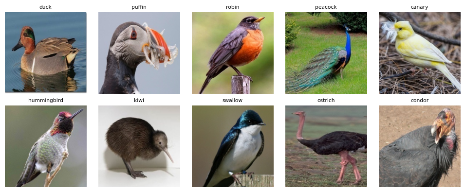
If we were to approach this problem using the techniques from Chapter 13, we would need to design a neural network architecture, choose appropriate hyperparameters, and train the model on our relatively small dataset. This would likely require extensive experimentation and might still produce mediocre results due to the limited training data available. Instead, we will use transfer learning to leverage the knowledge encoded in a model that has already been trained on millions of images.
Here, we will use the internal representations of a powerful, pre-built deep learning model as a jumping-off point for our own model. The final predictions from the existing model would not be very helpful because they predict categories that are not the same as ours. But, the internal representations of images are sufficiently generic and meaningful to be a good starting point for our models. This approach is called transfer learning. It accounts, in one form or another, for the vast majority of use-cases of deep learning because the best models require very large amounts of training data and compute time.
Python is the de facto language for machine learning, deep learning, and AI research. It is one of the key reasons we are using it in this revised text. As a result, there are fantastic ready-to-use libraries to build, run, and load deep learning models. We have wrapped up one of these models in the function called ViTEmbedder (the code to create it uses pytorch and is given in full in the notebooks). It implements Google’s Vision Transformer (ViT) model, which was trained on a dataset of 14 million images with a total of 21,843 classes. We will use the values in the internal representation of the final model that come right before the predictions of the classes in the original. Here is all we need to load (and, if not already grabbed, download) the model:
vit = ViTEmbedder()The Vision Transformer model works by dividing an image into a grid of patches, treating each patch as a token similar to how language models treat words. These patches are then processed through multiple transformer layers that allow the model to learn relationships between different parts of the image. The result is a rich representation that captures both local details and global structure.
Calling the model on an image path returns a sequence of 768 numbers. These numbers, called an embedding, form a compact representation of the image’s content. Two images that are visually similar will have embeddings that are close together in this 768-dimensional space, while dissimilar images will have embeddings that are far apart. We can see an example on the first few bird images:
(
    birds
    .head(5)
    .with_columns(
        vit = c.filepath.map_elements(
            vit, return_dtype=pl.List(pl.Float32)
        )
    )
)
shape: (5, 5)
| label | filepath | index | vit | siglip |
|---|---|---|---|---|
| str | str | str | list[f32] | list[f64] |
| "canary" | "media/birds10/00000.png" | "test" | [0.017947, -0.0305, … 0.003526] | [-0.00611, -0.042975, … -0.031687] |
| "canary" | "media/birds10/00001.png" | "train" | [0.024804, -0.045255, … -0.007233] | [-0.033767, -0.011978, … -0.020352] |
| "canary" | "media/birds10/00002.png" | "train" | [0.050587, -0.024486, … 0.029895] | [-0.033664, -0.008117, … -0.01725] |
| "canary" | "media/birds10/00003.png" | "train" | [0.047036, -0.038993, … -0.008446] | [-0.010029, -0.018192, … -0.009869] |
| "canary" | "media/birds10/00004.png" | "train" | [0.036349, -0.02734, … -0.018185] | [-0.027327, 0.003568, … -0.033407] |
Computing embeddings for all images in the dataset takes some time, so we have precomputed these values and stored them in a Parquet file. Parquet is a columnar storage format that is particularly well-suited for analytical workloads. Unlike CSV files, Parquet preserves data types exactly, handles nested structures like lists efficiently, and compresses data effectively. This makes it an excellent choice for storing embeddings, which are arrays of floating-point numbers that would be awkward to represent in CSV format. Reading the precomputed embeddings is straightforward:
birds = pl.read_parquet("data/birds10.parquet")
birds
shape: (1_555, 5)
| label | filepath | index | vit | siglip |
|---|---|---|---|---|
| str | str | str | list[f64] | list[f64] |
| "canary" | "media/birds10/00000.png" | "test" | [0.017947, -0.0305, … 0.003526] | [-0.00611, -0.042975, … -0.031687] |
| "canary" | "media/birds10/00001.png" | "train" | [0.024804, -0.045255, … -0.007233] | [-0.033767, -0.011978, … -0.020352] |
| "canary" | "media/birds10/00002.png" | "train" | [0.050587, -0.024486, … 0.029895] | [-0.033664, -0.008117, … -0.01725] |
| "canary" | "media/birds10/00003.png" | "train" | [0.047036, -0.038993, … -0.008446] | [-0.010029, -0.018192, … -0.009869] |
| "canary" | "media/birds10/00004.png" | "train" | [0.036349, -0.02734, … -0.018185] | [-0.027327, 0.003568, … -0.033407] |
| … | … | … | … | … |
| "swallow" | "media/birds10/01550.png" | "train" | [-0.022461, -0.025098, … -0.061945] | [-0.022029, -0.008476, … -0.003879] |
| "swallow" | "media/birds10/01551.png" | "train" | [-0.000212, -0.003448, … -0.058042] | [-0.02476, -0.016369, … 0.003875] |
| "swallow" | "media/birds10/01552.png" | "train" | [-0.012531, -0.006788, … -0.047077] | [-0.022153, 0.00765, … -0.011152] |
| "swallow" | "media/birds10/01553.png" | "test" | [-0.007587, -0.053535, … -0.046395] | [-0.005022, 0.00878, … -0.017564] |
| "swallow" | "media/birds10/01554.png" | "train" | [-0.01325, -0.032453, … -0.050751] | [-0.015117, -0.00685, … -0.029756] |
Notice that the dataset now includes a vit column containing the 768-dimensional embedding for each image. With these embeddings in hand, we can now train a classifier using the techniques from earlier chapters. The key insight is that we are not training a deep neural network from scratch. Instead, we are using logistic regression on the embedding features, which is computationally cheap and requires far less data than end-to-end deep learning.
model = (
    birds
    .pipe(
        DSSklearn.logistic_regression_cv,
        target=c.label,
        features=[c.vit],
        stratify=c.label,
        l1_ratios=[0],
        solver="saga"
    )
)
The results are impressive given how little effort we put into the modeling process. We simply extracted pre-trained embeddings and applied logistic regression with cross-validation to select the regularization strength.
model.score(){'train': 1.0, 'test': 1.0}The confusion matrix shows us which species are most often confused with each other. This can provide insight into the structure of the problem and potentially guide data collection if we wanted to improve performance further. In this case we see that the model does not make a single error on our dataset!
model.confusion_matrix()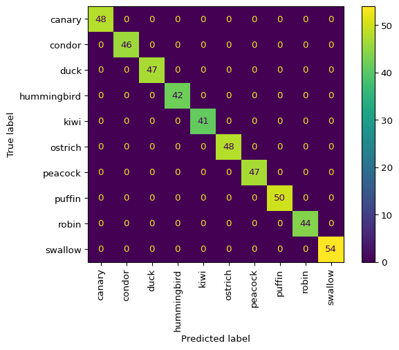
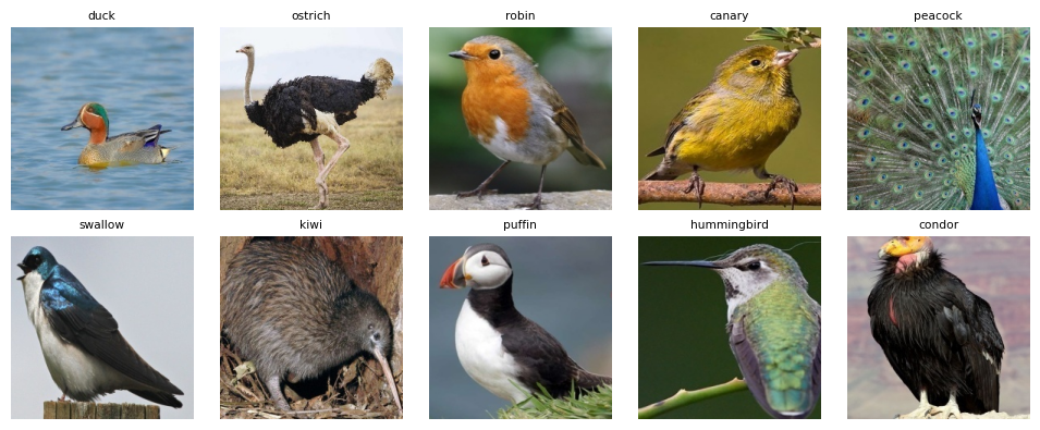
To better understand what the model has learned, we can examine the images that the model is most confident about. These are the examples where the predicted probability for the correct class is highest. Looking at these high-confidence predictions helps verify that the model is attending to meaningful features of the birds rather than artifacts of the images.
(
    birds
    .with_columns(
        model.predict_proba()
    )
    .filter(c.index == "test")
    .sort(c.prob_pred_, descending=True)
    .group_by(c.label)
    .agg(
        filepath = c.filepath.first()
    )
    .pipe(DSImage.plot_image_grid, ncol=5)
)
Beyond classification, embeddings can also be visualized to understand the structure of our data. Dimensionality reduction techniques like UMAP (Uniform Manifold Approximation and Projection) can project the 768-dimensional embeddings down to two dimensions while preserving the relative distances between points. This allows us to see how the different bird species cluster in the embedding space.
(
    birds
    .pipe(
        DSSklearn.umap,
        features=[c.vit]
    )
    .predict(full=True)
    .pipe(ggplot, aes("dr0", "dr1"))
    + geom_point(aes(color="label"))
)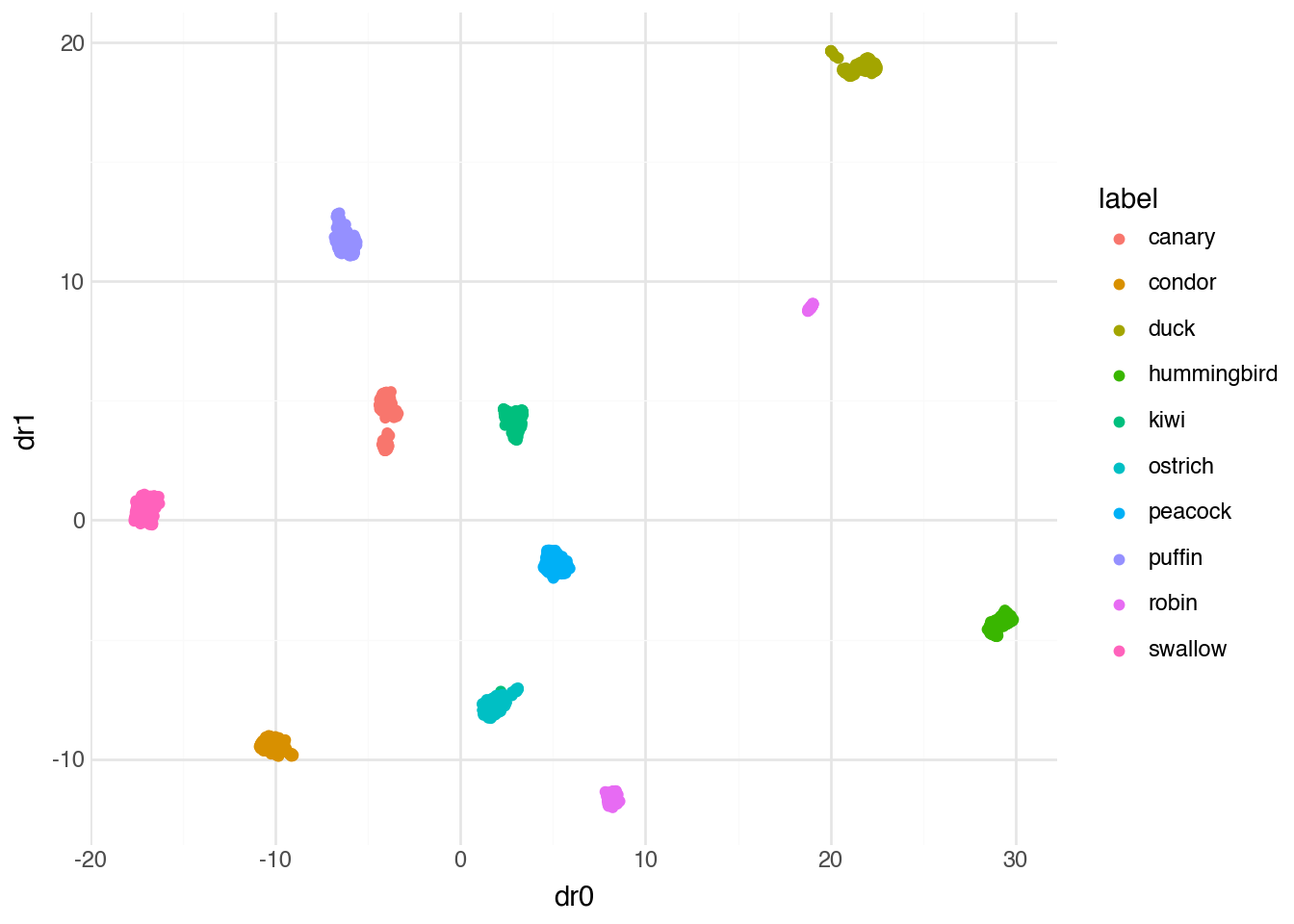
Notice that the UMAP projection does an incredibly good job of separating the categories. Images of the same species cluster tightly together, while different species form distinct groups. This visualization confirms that the ViT embeddings capture meaningful information about bird species, information that was never explicitly part of the original model’s training objective but emerged naturally from learning to classify images more generally.
15.4 Zero-shot Learning
Let’s see another way that we can extend transfer learning using an even newer class of deep learning models called zero-shot models. These work, at least conceptually, by allowing us to do classification on a new dataset with data that the original model may never have seen with no additional training data needed. The idea sounds almost magical: we can classify images into categories without ever showing the model any labeled examples of those categories.
Zero-shot learning became practical with the development of multimodal models that learn to connect images and text in a shared embedding space. These models are trained on massive datasets of image-caption pairs scraped from the internet. By learning to match images with their textual descriptions, the models develop an understanding of concepts that can be expressed in natural language. To classify a new image, we simply compare its embedding to the embeddings of text descriptions of each possible category.
We will use a model called SigLIP (Sigmoid Language-Image Pre-training), which represents the current state of the art in this type of approach. Like ViT, we have wrapped the model in a convenient interface that handles loading and embedding.
siglip = SigLIPEmbedder()The SigLIP model can embed both images and text into the same space. Images that match a textual description will have embeddings that are close together, measured by the dot product of their embedding vectors. Let’s start with a simple example: we will create a text embedding for “a photo of a canary” and see which images in our dataset are most similar to this description.
embed = (
    pl.DataFrame({"text": ["a photo of a canary"]})
    .with_columns(
        siglip_txt = c.text.map_elements(
            siglip.embed_text,
            return_dtype=pl.List(pl.Float32)
        )
    )
)
Now we can compute the similarity between this text embedding and every image in our dataset. The dot product of two normalized vectors measures how aligned they are: values close to 1 indicate high similarity, while values close to 0 indicate the vectors are nearly orthogonal (unrelated).
(
    birds
    .join(embed, how="cross")
    .with_columns(
        sim_score = dot_product(c.siglip, c.siglip_txt)
    )
    .sort(c.sim_score, descending=True)
)
shape: (1_555, 8)
| label | filepath | index | vit | siglip | text | siglip_txt | sim_score |
|---|---|---|---|---|---|---|---|
| str | str | str | list[f64] | list[f64] | str | list[f32] | f64 |
| "canary" | "media/birds10/00092.png" | "train" | [0.02978, -0.047476, … 0.033946] | [-0.031486, -0.00417, … -0.034138] | "a photo of a canary" | [-0.013163, 0.00856, … -0.006386] | 0.174141 |
| "canary" | "media/birds10/00025.png" | "test" | [0.034456, -0.036724, … 0.01517] | [-0.012494, -0.006824, … -0.011134] | "a photo of a canary" | [-0.013163, 0.00856, … -0.006386] | 0.168272 |
| "canary" | "media/birds10/00119.png" | "train" | [0.040854, -0.038557, … 0.013647] | [-0.023419, -0.008008, … -0.032821] | "a photo of a canary" | [-0.013163, 0.00856, … -0.006386] | 0.166631 |
| "canary" | "media/birds10/00115.png" | "test" | [0.020037, -0.035357, … 0.006308] | [-0.018599, -0.002016, … -0.018126] | "a photo of a canary" | [-0.013163, 0.00856, … -0.006386] | 0.164925 |
| "canary" | "media/birds10/00122.png" | "train" | [0.024512, -0.034228, … 0.011564] | [-0.031184, -0.00085, … -0.041639] | "a photo of a canary" | [-0.013163, 0.00856, … -0.006386] | 0.16463 |
| … | … | … | … | … | … | … | … |
| "duck" | "media/birds10/00393.png" | "test" | [-0.016794, -0.018484, … 0.031061] | [-0.03385, -0.008774, … -0.020661] | "a photo of a canary" | [-0.013163, 0.00856, … -0.006386] | -0.059658 |
| "duck" | "media/birds10/00404.png" | "test" | [-0.004223, 0.002329, … 0.016521] | [-0.027971, 0.003032, … -0.035659] | "a photo of a canary" | [-0.013163, 0.00856, … -0.006386] | -0.060996 |
| "condor" | "media/birds10/00272.png" | "train" | [-0.046735, -0.034367, … -0.003293] | [0.008176, 0.001546, … 0.007645] | "a photo of a canary" | [-0.013163, 0.00856, … -0.006386] | -0.062812 |
| "duck" | "media/birds10/00423.png" | "train" | [0.004472, -0.02733, … 0.018769] | [-0.042206, 0.008924, … -0.033317] | "a photo of a canary" | [-0.013163, 0.00856, … -0.006386] | -0.065547 |
| "condor" | "media/birds10/00308.png" | "test" | [-0.057108, 0.000503, … -0.003844] | [0.003084, 0.027618, … 0.002365] | "a photo of a canary" | [-0.013163, 0.00856, … -0.006386] | -0.075263 |
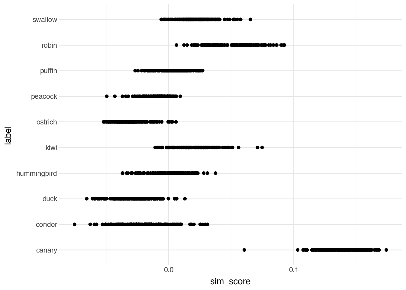
Visualizing the similarity scores by bird species shows that canary images indeed have the highest similarity to our “a photo of a canary” text prompt. This demonstrates that the model has learned a meaningful connection between the visual appearance of canaries and the word “canary” without us ever explicitly teaching it this connection.
(
    birds
    .join(embed, how="cross")
    .with_columns(
        sim_score = dot_product(c.siglip, c.siglip_txt)
    )
    .pipe(ggplot, aes("sim_score", "label"))
    + geom_point()
)
To perform zero-shot classification on the entire dataset, we need to create text embeddings for all of our bird species categories. We can then assign each image to the category whose text embedding it is most similar to. This process requires no training data at all; we are simply leveraging the knowledge the model acquired during its original pre-training.
embed = (
    birds
    .select(text = c.label.unique())
    .with_columns(
        siglip_txt = c.text.map_elements(
            siglip.embed_text, return_dtype=pl.List(pl.Float32)
        )
    )
)
For each image, we compute its similarity to every category label, then select the label with the highest similarity as the predicted class. The classification rate tells us how often this zero-shot approach correctly identifies the bird species.
(
    birds
    .join(embed, how="cross")
    .with_columns(
        sim_score = dot_product(c.siglip, c.siglip_txt)
    )
    .sort(c.sim_score, descending=True)
    .group_by(c.filepath)
    .head(1)
    .select(class_rate = (c.label == c.text).mean())
)
shape: (1, 1)
| class_rate |
|---|
| f64 |
| 0.998714 |
While the zero-shot accuracy makes a few errors (in comparison to the model above), it is remarkable that we can achieve any reasonable classification performance without a single labeled training example, let alone such a strong classification rate on the testing data. This approach is particularly valuable when labeled data is expensive or impossible to obtain, there are a very large number of categories, or when we need to quickly prototype a classification system for new categories.
Let’s examine the images that the zero-shot classifier got wrong. Understanding these errors can provide insight into the model’s limitations and the ambiguity inherent in visual classification.
(
    birds
    .join(embed, how="cross")
    .with_columns(
        sim_score = dot_product(c.siglip, c.siglip_txt)
    )
    .sort(c.sim_score, descending=True)
    .group_by(c.filepath)
    .head(1)
    .filter(c.label != c.text)
    .with_columns(
        desc = pl.concat_str("label", "text", separator=" => ")
    )
    .pipe(DSImage.plot_image_grid, label_name="desc", ncol=3)
)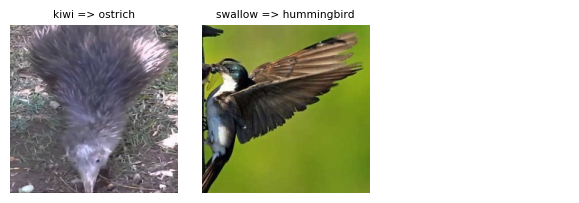
These two misclassifications involve birds in strange positions and that are cropped at the edges, cutting off import aspects that differentiate the species.
15.5 Text Embedding
The transfer learning approach we applied to images works equally well for text data. Just as image models learn to represent visual content in ways that transfer across tasks, language models learn to represent text in ways that capture semantic meaning. By extracting embeddings from a pre-trained language model, we can build text classifiers with minimal task-specific training.
For this section, we will use a dataset of movie reviews from IMDB. Each review is labeled as either positive or negative, and our goal is to predict the sentiment from the text content. This is the same task we approached in Chapter 13 using neural networks trained from scratch, which allows us to directly compare the transfer learning approach.
imdb = pl.read_parquet("data/imdb5k_pca.parquet")
imdb
shape: (5_000, 5)
| id | label | text | index | e5 |
|---|---|---|---|---|
| str | str | str | str | list[f64] |
| "doc0001" | "negative" | "In my opinion, this movie is n… | "test" | [-0.253192, 0.099743, … -0.000806] |
| "doc0002" | "positive" | "Loved today's show!!! It was a… | "test" | [0.280815, -0.064508, … -0.0273] |
| "doc0003" | "negative" | "Nothing about this movie is an… | "test" | [-0.179638, 0.171097, … 0.007573] |
| "doc0004" | "positive" | "Even though this was a disaste… | "train" | [0.300824, 0.027666, … -0.028764] |
| "doc0005" | "positive" | "I cannot believe I enjoyed thi… | "test" | [0.319154, 0.035425, … 0.001316] |
| … | … | … | … | … |
| "doc4996" | "positive" | ""Americans Next Top Model" is … | "test" | [0.305853, 0.026326, … 0.006194] |
| "doc4997" | "negative" | "It's very sad that Lucian Pint… | "train" | [0.217778, 0.283147, … -0.028361] |
| "doc4998" | "positive" | "Ruth Gordon at her best. This … | "train" | [0.373751, 0.076117, … -0.032517] |
| "doc4999" | "negative" | "I actually saw the movie befor… | "test" | [-0.073533, 0.10723, … 0.019535] |
| "doc5000" | "positive" | "I've Seen The Beginning Of The… | "test" | [0.147752, -0.095977, … -0.02008] |
The dataset includes precomputed embeddings from the E5 model, a powerful text embedding model designed specifically to produce representations suitable for downstream tasks like classification and semantic search. Like the image embeddings we used earlier, these text embeddings capture the semantic content of each review in a fixed-dimensional vector that can be used as input to any classifier.
Training a logistic regression model on these embeddings follows exactly the same pattern we used for the bird classification task. The only difference is the source of the embeddings: images of birds versus reviews of movies.
model = (
    imdb
    .pipe(
        DSSklearn.logistic_regression_cv,
        target=c.label,
        features=[c.e5],
        stratify=c.label,
        l1_ratios=[0],
        solver="saga"
    )
)
The performance using transfer learning noticeably exceeds what we achieved in Chapter 13 with neural networks trained from scratch. This improvement comes from the E5 model’s pre-training on vast amounts of text data, which gives it a sophisticated understanding of language that would be impossible to learn from our relatively small training set.
model.score(){'train': 0.9577142857142857, 'test': 0.9426666666666667}model.confusion_matrix()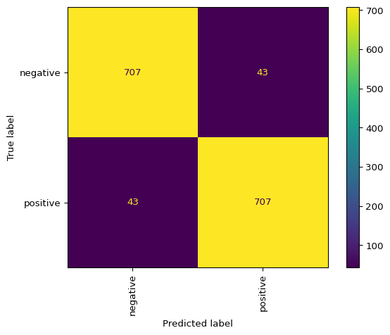
As with the bird images, we can visualize the embedding space using UMAP to see how positive and negative reviews cluster. Well-separated clusters indicate that the embeddings capture the sentiment distinction effectively.
(
    imdb
    .pipe(
        DSSklearn.umap,
        features=[c.e5]
    )
    .predict(full=True)
    .pipe(ggplot, aes("dr0", "dr1"))
    + geom_point(aes(color="label"))
)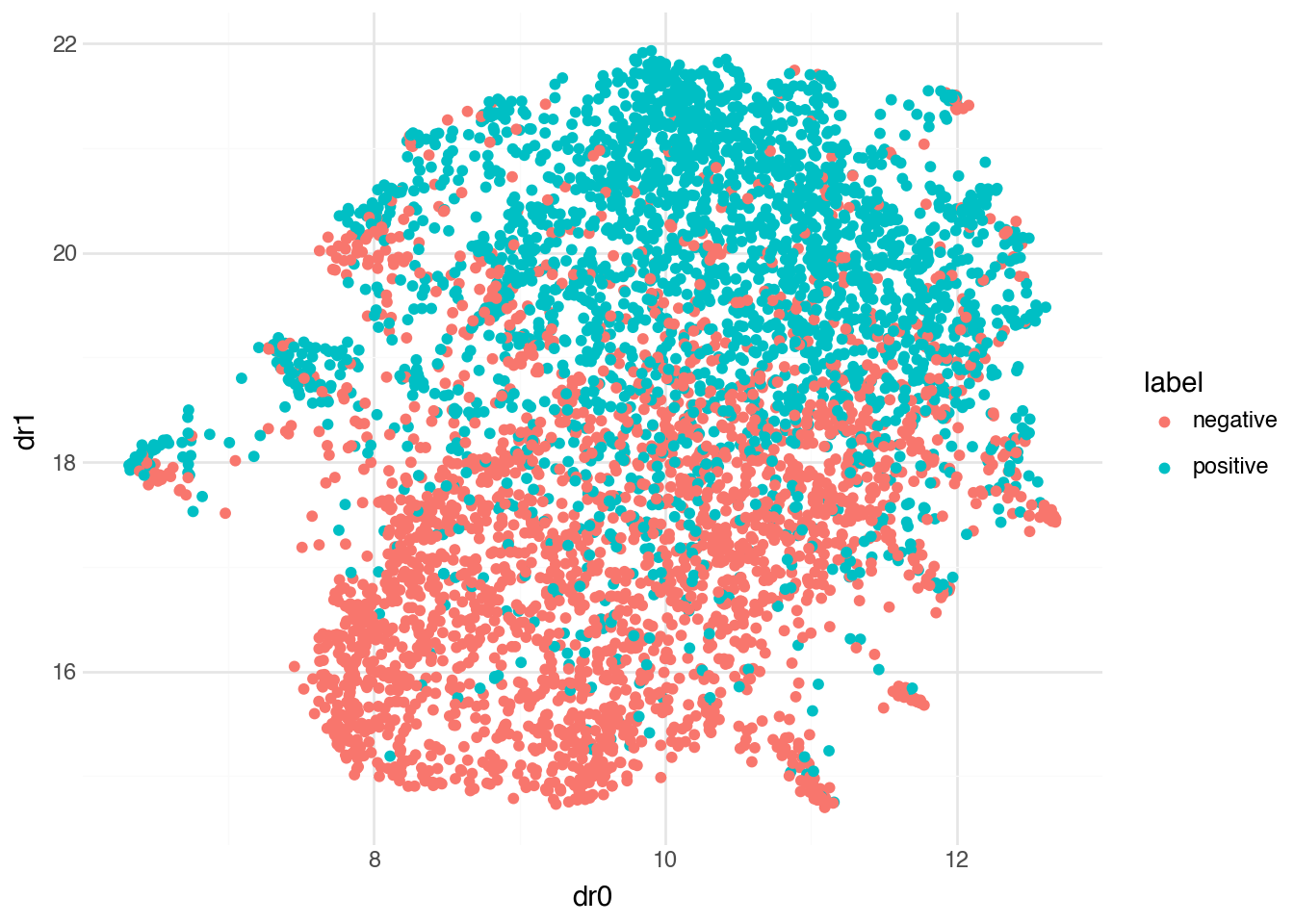
The clear separation between positive and negative reviews in this visualization explains why a simple logistic regression classifier performs so well: the embedding model has already done the hard work of mapping reviews into a space where sentiment is linearly separable.
15.6 Calling an API
Throughout this chapter, we have used pre-trained models that run locally on our computer. This gives us complete control over our data and allows us to process examples quickly once the models are loaded. However, the most powerful AI models available today are too large to run on typical hardware. These models, with billions or even trillions of parameters, require specialized infrastructure to operate and are typically accessed through web-based APIs.
Using an API to access AI capabilities represents another form of transfer learning. Instead of downloading model weights and running inference locally, we send our data to a remote server that processes it using state-of-the-art models and returns the results. This approach offers access to capabilities far beyond what we could run locally, at the cost of per-request pricing and the need to send data over the network.
Here is an example of using OpenAI’s API to classify a movie review. The API accepts natural language instructions, so we can describe the classification task in plain English rather than training a model.
client = OpenAI()

review_text = imdb.select("text").to_series()[0]

response = client.responses.create(
    model="gpt-5-mini-2025-08-07",
    input=(
        "Return only one word, either 'positive' or 'negative'" +
        "for this review:\n\n" +
        review_text
    )
)

label = response.output_text
label'negative'The simplicity of this approach is striking: we describe what we want in natural language, provide the input data, and receive a structured response. This zero-shot capability, combined with instruction-following, makes large language models incredibly versatile tools for data processing tasks that would traditionally require custom model development.
However, API-based approaches have important tradeoffs to consider. Each request incurs a cost, which can add up quickly when processing large datasets. Latency is higher than local inference because data must travel over the network. Privacy concerns may prevent sending sensitive data to external services. And the behavior of API models can change without notice as providers update their systems. For production applications with stable requirements and sufficient training data, local models trained via transfer learning often provide a better balance of cost, reliability, and performance.
15.7 Conclusions
Transfer learning has fundamentally changed how we approach machine learning problems. Rather than treating each task as a fresh challenge requiring massive datasets and extensive training, we can build on the knowledge captured in pre-trained models to achieve strong performance with minimal effort. This chapter demonstrated three complementary approaches to leveraging pre-trained models.
First, we used embeddings from vision and language models as features for traditional classifiers. This approach requires some labeled data but dramatically reduces the amount needed compared to training from scratch. The ViT embeddings for bird classification and E5 embeddings for sentiment analysis both yielded excellent results with simple logistic regression classifiers. The key insight is that modern embedding models transform raw inputs into representations where the concepts we care about are often linearly separable.
Second, we explored zero-shot classification with multimodal models like SigLIP. By learning to connect images and text in a shared embedding space, these models can classify images into arbitrary categories described in natural language without any task-specific training. While accuracy may be lower than fine-tuned approaches, zero-shot methods enable rapid prototyping and handle scenarios where labeled data is unavailable.
Third, we briefly examined how external APIs provide access to capabilities beyond what we can run locally. Large language models accessible through APIs can perform classification and many other tasks given only natural language instructions. This represents the extreme end of transfer learning, where we leverage models trained on essentially all available text and images to perform specific tasks on demand.
The choice among these approaches depends on the specific requirements of each application. When labeled data is plentiful and consistent performance is critical, traditional embedding plus classifier approaches offer the best balance. When exploring new problems or working with limited labels, zero-shot methods provide a quick baseline. And when tasks require sophisticated language understanding or domain knowledge, API-based models may offer capabilities that local approaches cannot match.
As pre-trained models continue to improve, the bar for what can be accomplished with transfer learning keeps rising. Tasks that once required extensive custom development can now be solved by combining off-the-shelf embeddings with simple classifiers. This democratization of machine learning capabilities is one of the most significant developments in the field, making powerful AI accessible to practitioners who may not have the resources for large-scale model training.