import numpy as np
import polars as pl

from funs import *
from plotnine import *
from polars import col as c
theme_set(theme_minimal())

import torch.nn as nn
import torch.optim as optim

mnist = pl.read_csv("data/mnist_1000.csv")13 Deep Learning
13.1 Setup
Load all of the modules and datasets needed for the chapter. We load two submodules of the torch module to build neural network models. The mnist dataset contains a sample of 1,000 images of handwritten digits from the well-known MNIST collection. Full details are available in Chapter 22.
13.2 Introduction
The main idea behind deep learning is that instead of building a model, such as linear regression, that goes from the inputs to the predictions, we should generate intermediate results that summarize the important information in the inputs. The summarized information can then be used to produce the final predictions. The idea can be expanded to many layers of intermediate representations. This is where the term “deep” come from, indicating that there is a large distance between the things we put into the model and the things that come out of it. The earliest deep models drew from biological analogies to neurons in the brain, which is why the models also became known as neural networks. These ideas have been incredibly powerful, perhaps the single most important idea in computer science in the last 50 years, and have been behind almost all of the growth in machine learning and AI over the past two decades, including the rise of generative text models such as ChatGPT.
The power of deep learning is most apparent in application domains where the input data is only connected to the things we want to know about the data in a complex and/or abstract way. This is true, for example, with text analysis where individual letters only have meaning when put together in specific patterns and orders. The same goes for the air pressure measurements that are recorded in sound data and the individual pixels that represent images. A sequence of sound pressures gets interpreted as a specific song only through a complex relationship that is hard to explain but easy for our ears and brains to decode. The inner representations within a deep learning model work to transform the raw data into things that more closely have a connection to the things they represent.
Training deep learning models requires more hands-on background knowledge than kinds of models we saw in Chapters 13 and 14. While there is a lot of theory of computational depth in linear and logistic regression models, once experts have coded the algorithms to learn from data we can (mostly) apply them without understanding the mechanics of how the models determine the final weights. This is not so with deep learning because there are far too many different ways that different sets of intermediate results could produce the same predictions. Choosing “good” representations is the key to making the model work well on data that it has not been trained on. This is something that is attainable by anyone reading this book (it’s not magic), but requires some practice and time.
13.3 MNIST Data
To understand the true power of deep learning we need to work with a dataset where there is a disconnect between the information contained in the object and the raw format of the data that we are given. This, for example, is the case with text, image, video, and sound data. There is a wide gap between the data stored on one hand in the individual pixels of an image, characters in a text, or sound pressure at a specific millisecond and the semantic meaning represented by these objects when processed by the human perceptive system.
In order to better understand how this works, we will work in this chapter with a subset of the MNIST (Modified National Institute of Standards and Technology database) hand-written digits dataset. This is one of the earliest popular image processing datasets. It consists of small, standardized images of hand-written digits from 0 to 9. The goal is to build a supervised model that recognizes which digit is written based on the image. All of the image datasets in this text use a format where we have metadata about the images in one table. This table includes a filepath column that contains the location of each of the image files. In this case, each image is a greyscale file of a square image that is 28 pixels tall and wide. Here is the dataset:
mnist
shape: (1_000, 3)
| label | filepath | index |
|---|---|---|
| i64 | str | str |
| 3 | "media/mnist_1000/00000.png" | "test" |
| 9 | "media/mnist_1000/00001.png" | "test" |
| 9 | "media/mnist_1000/00002.png" | "train" |
| 8 | "media/mnist_1000/00003.png" | "test" |
| 8 | "media/mnist_1000/00004.png" | "train" |
| … | … | … |
| 4 | "media/mnist_1000/00995.png" | "train" |
| 4 | "media/mnist_1000/00996.png" | "train" |
| 6 | "media/mnist_1000/00997.png" | "test" |
| 4 | "media/mnist_1000/00998.png" | "train" |
| 7 | "media/mnist_1000/00999.png" | "test" |
We have a helper function called DSImage.plot_image_grid that allows us to see a collection of the images from within Python along with their labels. Here is an example of what the data looks like for 30 randomly selected images.
DSImage.plot_image_grid(mnist.sample(30))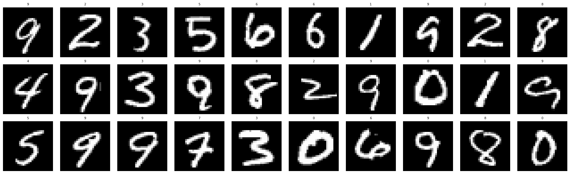
In order to load the data into Python, we have another helper function called DSTorch.load_image that takes the dataset and some parameters and generates objects corresponding to the features and responses of the data. We have both the data split into a training and testing set as well as the complete original data. The latter is useful if we later want to add information back into the mnist table.
X, X_train, X_test, y, y_train, y_test, cn = DSTorch.load_image(
    mnist, scale=True, flatten=True
)
Notice that we set the option flatten to True above. This takes the pixel data from the images and converts them to a single vector that has no implicit encoding of the shape of the image. In this case, this means that the 28-by-28 grid of pixel intensities has been converted into a single string of \(28 * 28 = 784\) values. We can see the shape of the X object below.
X.shapetorch.Size([1000, 784])All of the objects returned by DSTorch.load_image other than cn (the category names) are special objects called a Tensor created by the torch library. These are the formats that we will need to run deep-learning models in Python. The category names are returned because the y Tensor needs to be integer codes rather than the names of the labels. In the special case of MNIST these are the same (the digits are already integer codes). In nearly every other application this will be different and having the original names will be very helpful.
13.4 Dense Neural Networks
Let’s say we have a dataset with \(n\) features that we want to use to predict an output. We’ve seen how to do linear regression with a linear combination of the parameters. We can modify this slightly by creating an intermediate value \(h\) that is a linear combination in exactly the same way and then produce the prediction for the output \(y\) as a simple linear combination of \(h\). Mathematically, we can write this as:
\[ \begin{aligned} h &= \beta_0 + \beta_1 \cdot x_1 + \beta_2 \cdot x_2 + \cdots + \beta_n \cdot x_n \\ y &= \gamma_0 + \gamma_1 \cdot h \end{aligned} \]
There are a few things to take note of here. First of all, the model as written is not fundamentally any different than linear regression. A linear combination of linear combinations is just another linear combination. We simply have more ways of getting to the same output. The second thing is that the value of \(h\) is not something we actually observe in the data. It is only an intermediate value that helps us go from the input values \(x_j\) to the output value \(y\). We use the letter \(h\) here because this value relates to a hidden state of the model in the sense that no data we observe is directly related to it.
In order to do something that is not possible with normal regressions, we need to add something non-linear (not just adding and multiplying constants) into the model. The typical way to do this is to add a pre-determined function that gets applied to the result before creating the value \(h\). This function is called an activation function. It is often written with the symbol \(\sigma(\cdot)\) (sigma) because the earliest models used a sigmoid function for this. We can modify our equation as follows.
\[ \begin{aligned} h &= \sigma\left(\beta_0 + \beta_1 \cdot x_1 + \beta_2 \cdot x_2 + \cdots + \beta_n \cdot x_n\right) \\ y &= \gamma_0 + \gamma_1 \cdot h \end{aligned} \]
Most models now use simpler activation functions than the sigmoid. The most common choice is a rectified linear unit (ReLU). While the name sounds complicated, the function is actually very simple. It is equal to the identity function for positive inputs while mapping all negative values to zero. Mathematically, we can write this as:
\[ \text{ReLU}(z) = \max(0, z) \]
The key features of an activation function are that it must be differentiable at almost all points and it must be non-linear. The ReLU satisfies both requirements while being computationally efficient to evaluate.
We can visually think about the mathematical formulation we now have as a network diagram such as the one in Figure Figure 13.1. For every observation, we have a number associated with each of the inputs in the left. Then, if we know all of the slopes and intercepts defined by the model, we can compute the hidden state \(h\) and the output value \(y\).
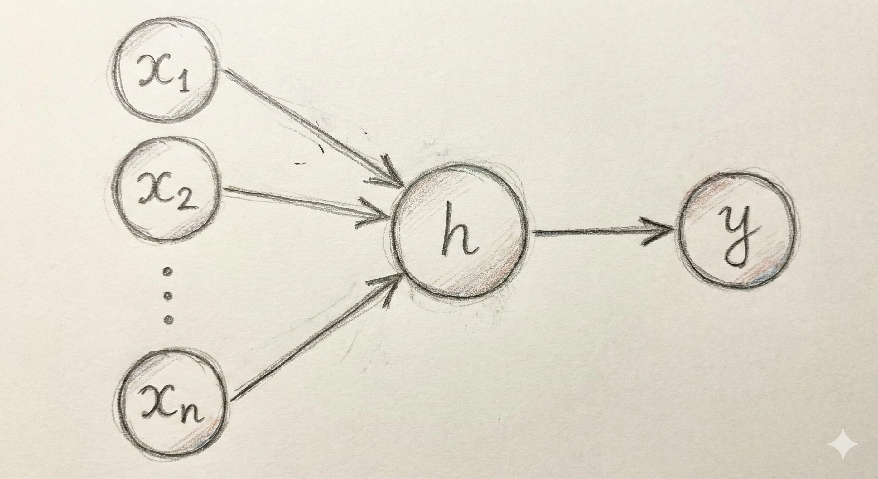
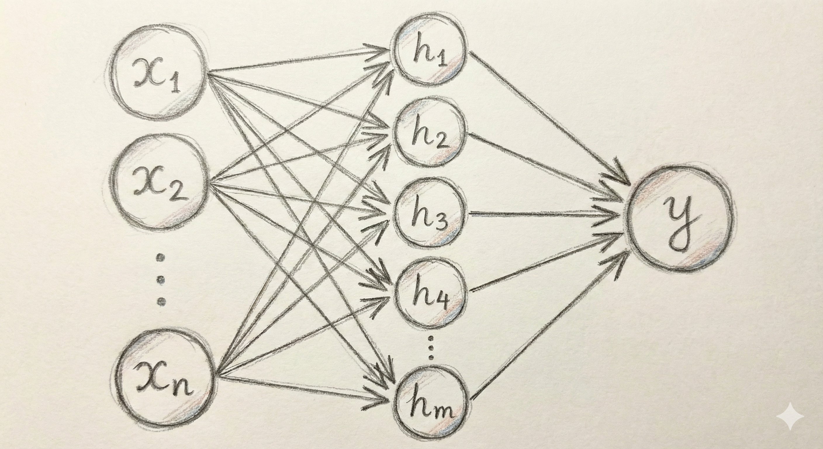
With the activation function we can now generate ways of producing estimates \(y\) from our input data that are not strictly the same as those from linear regression. However, we are still very constrained in the kinds of models we can build, and the overall complexity of what we can represent is essentially the same. In order to produce more complex models we need to include a larger set of hidden states, all of which are individual linear combinations of the inputs followed by the activation function. Then, the output \(y\) is a linear combination of all of these outputs. Below is a mathematical description of this model. Figure Figure 13.2 shows the corresponding visualization of adding more hidden states into our model.
\[ \begin{aligned} h_1 &= \sigma\left(\beta_{1,0} + \beta_{1,1} \cdot x_1 + \beta_{1,2} \cdot x_2 + \cdots + \beta_{1,n} \cdot x_n\right) \\ &\,\,\vdots \\ h_m &= \sigma\left(\beta_{m,0} + \beta_{m,1} \cdot x_1 + \beta_{m,2} \cdot x_2 + \cdots + \beta_{m,n} \cdot x_n\right) \\ y &= \gamma_0 + \gamma_1 \cdot h_1 + \cdots + \gamma_m \cdot h_m \end{aligned} \]
The model above is an example of the basic building blocks of a dense, shallow neural network. A very-well known result about neural networks shows that given enough hidden states, any well-behaved real-valued function of \(n\) dimensions can be approximated by such as model [1]. This property makes neural networks—even simple, shallow ones—a type of estimator known as a universal approximator.
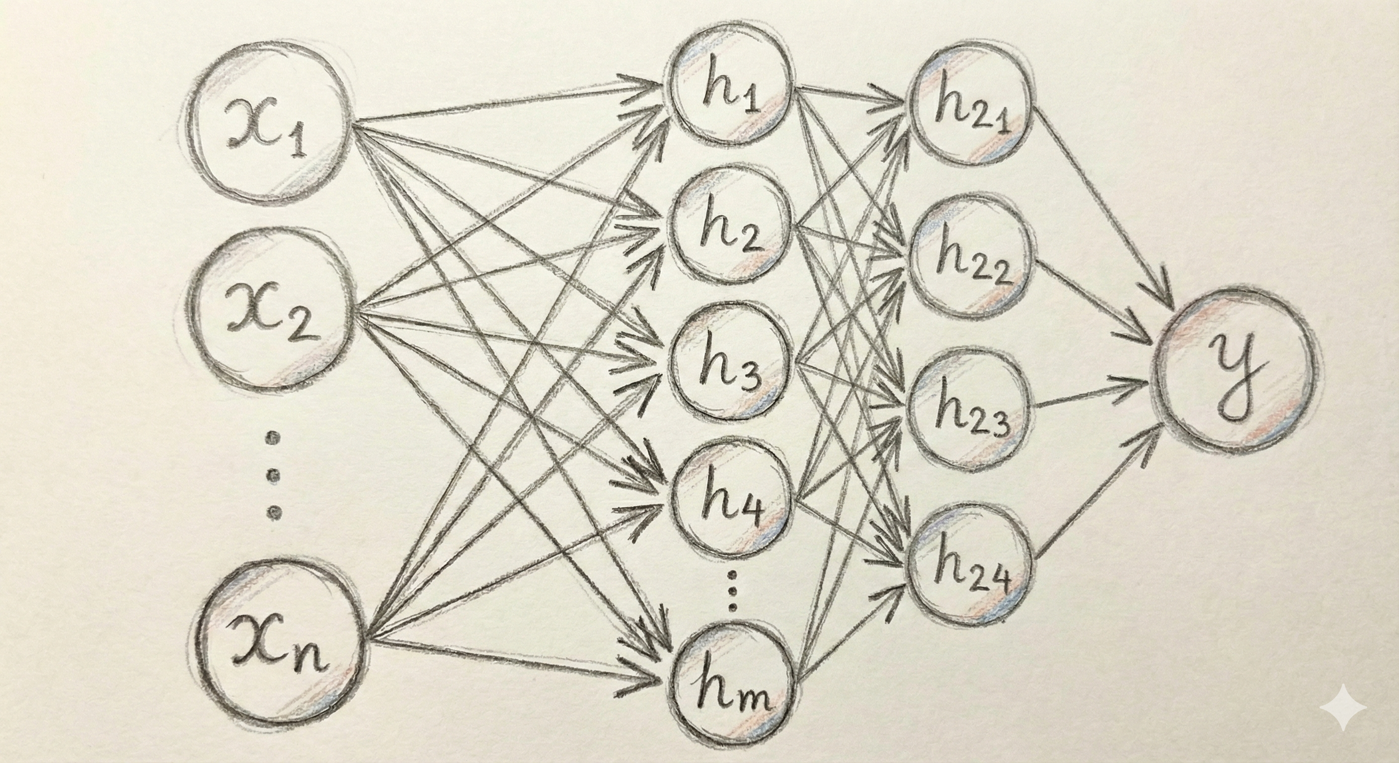
In order to see the real power of neural networks, we need to expand the model not just by the number of hidden states, but also by the number of hidden layers themselves. In other words, we can create a collection of hidden intermediate values that are combinations for the hidden values we created in the first layer and then use these second-order hidden layers to construct the output. We won’t attempt to write this out mathematically because the notation is already getting complicated. But, we can visualize this fairly straightforwardly as shown in Figure Figure 13.3.
We can continue in the same way by increasing the number of layers and adjusting the number of hidden states in each. As we increase the number of layers (the exact cut-off is debated; certainly after 10) we arrive at a deep neural network. It turns out that while even a one-hidden layer model can approximate any function, it is much quicker to approximate a function increasing the number of layers rather than the number of states within a layer. At the same time, it becomes more and more difficult to learn how to make the model do so, particularly when we are using large complex training data. In the next section we will investigate how we actually train these models using data.
Interpreting parameters
Unlike linear regression, where each coefficient directly measures the effect of a one-unit change in a predictor on the response, the parameters in a neural network have no straightforward interpretation. The weights connecting one hidden layer to another describe relationships between intermediate representations that have no direct connection to either the original inputs or the final output. Combined with the non-linear activation functions applied at each layer, it becomes essentially impossible to understand what any individual parameter does in a network of even modest size. This is why neural networks are sometimes called black-box models. We can observe what goes in and what comes out, but the internal workings remain opaque. Various research efforts have attempted to interpret neural network representations, with some success in specific domains like image classification, but this remains an active and challenging area of study.
Before we continue, it will be useful to modify our visual concept of a neural network beyond the complex web of circles and arrows that we have used so far. Instead of thinking about each hidden state as a separate entity, it will be much more scalable to think about each layer as a concrete unit. The typical way that you will see neural networks described in papers and in code is through the format shown in Figure Figure 13.4. This abstraction explains all of the information that we need to know other than the size of the input and the number of hidden states in each linear unit. Once we specify those, the model is completely described by this relatively simple diagram.
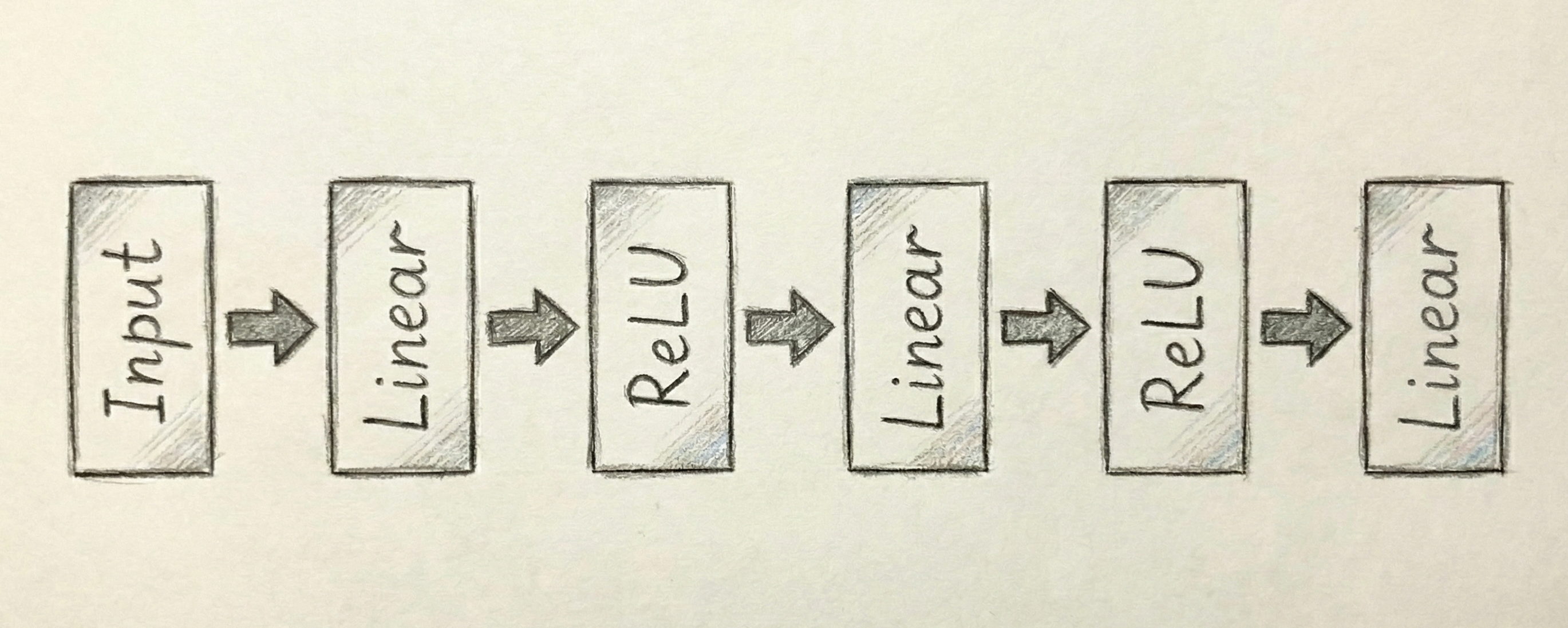
One thing that become clear with the abstract form of the neural network is that the process of going from the last hidden layer to the output is structurally the same as creating any of the internal hidden layers. In other words, these are all just linear units that consist of a linear combination of all the output from the previous states. The only difference is that the final Linear unit for a regression problem would always have only a single output that corresponds with the value we want to predict.
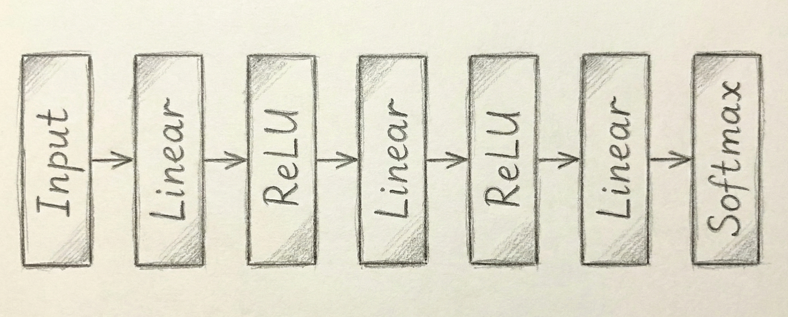
Almost all of the deep learning tasks we will look at involve classification. The fact that the output is structurally no different from the other layers indicates a way to using this to easily extend to classification. We can change the last layer to output one prediction for each category rather than only a single number. Then, we can apply a special activation function called as Softmax that turns a collection of number into a valid set of probabilities (all non-negative numbers that sum to one). Figure Figure 13.5 illustrates how this can be seen as one additional layer on the neural network.
We will continue to see throughout this chapter that deep neural networks can be extended by adding new layer types and combinations to work with increasingly large and complex datasets.
13.5 Stochastic Gradient Descent
When we introduced linear regression in Chapter 10 it was mentioned that the slopes and intercepts in the model were fit using ordinary least squares (OLS). In other words, we find the parameters that minimize the sum of squared differences between the model predictions and the observed data. There is a well known formula for solving OLS and we didn’t go any more into the computational details. We let statsmodels compute the values for us and moved on to the next step. When discussing penalized regression and gradient boosted trees in Chapter 11 we mentioned a few more details but still avoiding discussing too many computational details about the process. There are excellent algorithms already coded into sklearn that are able to find the optimal solutions in a straightforward way with no manual intervention. Neural networks are computationally much more complicated and will require some understanding of the way they are trained with data.
We will motivate the technique used in training neural networks with an easy to visualize one-dimensional example of trying to minimize a relatively smooth function. Of course, the ideal way to find the minimum of a function is to compute its derivative and determine where this derivative is equal to zero. In many cases, though, it is not possible to compute the derivative for all of the points and even when we can it may not be possible to figure out at what points that function is equal to zero. An alternative is to do something iterative: we start at an initial guess, compute measurements about the function in a small neighborhood of this point, and then use this information to find a new point that should be closer to the optimal value. We will look at a few different approaches of this type using a single function where our initial guess is near -2.
To start, we will compute the first and second derivative of the function at our initial starting point. This allows us to construct a quadratic approximation of the function. A quadratic function will always “turn around” somewhere. In other words, there will be an easy to compute minimum for the approximation of this approximation of the function. A straightforward approach is, therefore, to jump to the minimum of this approximation and then start the process all over again. We can do this until the process converges to a point, which it does in our example very quickly.
The technique above is called a second-order method because it uses the second derivative of the function to compute the minimum value. These techniques are very fast and for functions with unique minima have strong convergence results. Second-order methods are used throughout statistics and the sciences as the go-to method when there are no analytic solutions available, as is often the case when we go beyond the most basic techniques. Unfortunately, these are not feasible for training neural networks. The higher-dimensional analog of a second-derivative is a Hessian matrix, which in \(d\) dimensions requires \(d^2\) parameters. Modern neural networks often have dozens of billions of parameters. Storing a single Hessian matrix would take hundreds of Exabytes, or approximately 1 million hours of HD video. Clearly this is not a practical approach for such large models even if we had enough data to reliably compute the Hessian matrix, which we do not.
An alternative is to use a first-order method that is based only on the first derivative of the function at a given point. The multidimensional equivalent is the gradient. It requires only \(d\) parameters in \(d\) dimensions (one partial derivative for each dimension) and is therefore reasonable to both compute and store. The difficulty is that the derivative approximates a function by a line. This will tell us which direction to go in to find the minimum. By way of the slope, it may possibly also give some idea of how fast it is descending. However, since a line never turns around we have no idea how far to go in the direction of the derivative. The standard solution is to pick a positive value represented by \(\eta\) (eta) called the learning rate. We then update our guess of the optimal value by using the following formula (the negative sign because we are moving in the opposite direction of the derivative when minimizing the function):
\[ x \rightarrow x - \eta \times \frac{d}{dx}(x) \]
This technique is called gradient descent. The visualization below shows an example of gradient descent with a relatively small value of \(\eta\). The algorithm eventually finds the minimum, but only after taking a large number of small steps.
In the example below we use a larger value for \(\eta\). The first two steps are approach the minimum much quicker, but the increased learning rate eventually causes the estimates to bounce back and forth on other side of the minimum value and it never seems to completely converge to the optimal point (at least during the cycle of the simulation).
The two examples above illustrate how the choice of the learning rate greatly affects the ability of even a simple one-dimensional example to converge to a minimum value. Too low and we do not move fast enough; too large and we bounce around the minimum value and never converge. These do illustrate, though, two ways of trying to improve the performance of gradient descent. First of all, we can slowly decrease the learning rate over time. Bigger steps are great to make quick progress to decent values and then smaller steps can be used to refine the best parameters in a local neighborhood. Secondly, we can introduce a momentum term that keeps track of how the derivatives change over time. When, as in the first case, they continue to increase in the same direction we can pick up the pace of the steps. In the second case, the derivatives keep shifting directions, indicating that we should take very small steps to center into the minimum value. We can describe this by setting a momentum factor \(\mu\), keeping track of a velocity value \(v\) and updating as follows:
\[ \begin{aligned} v &\rightarrow \mu \times v - \eta \times \frac{d}{dx}(x) \\ x &\rightarrow x + v \\ \end{aligned} \]
A visualization of this is given below, where we see that the convergence happens quicker than in the low learning rate case but does not overshoot the target as in the high learning rate case.
Note that all of the methods introduced here, including the powerful second-order methods, have the possibility of getting stuck in a local minimum, such as the one in our example around \(x=1\). For example, below is a visualization in which our momentum term is turned too high and we ultimately get into the second minima.
While the models we saw in previous chapters have convex functions that define their optimal values, the complex nature of the parameters in neural networks causes them to have a very large number of local optima. This means that we never find the true minimum. Rather, the goal is simply to find a value of the parameters that produces reasonably predictive results.
We’ve talked a lot in the abstract about optimization here. How does this actually get put into practice with neural networks? As with OLS or logistic regression, we can train a neural network with training data to find the parameters (the slopes and intercepts in all of the hidden layers) that attempt to minimize the RMSE or classification error rate. This is done using a modified version of the methods introduced above called stochastic gradient descent (SGD). The only core difference is that rather than using all of the (often very large) data to determine the derivatives at each step, we instead take a small step using data from only a small set of the observations in the training data. We do this over and over again until we have used every data point once, called an epoch, and then start over again.
Backpropagation
Computing the gradient in a neural network requires determining how changes in each parameter affect the final loss function. This is complicated because parameters in early layers influence the output only indirectly, through many subsequent layers. The solution is an algorithm called backpropagation, which applies the chain rule from calculus systematically through the network. Starting from the output layer and working backward toward the input, backpropagation computes how much each parameter contributed to the prediction error. For a given batch of training examples, we first run the forward pass to compute predictions, then run the backward pass to compute gradients, and finally update the parameters using those gradients. Modern deep learning libraries like PyTorch handle backpropagation automatically, building a computational graph during the forward pass that records all operations, then traversing this graph in reverse to compute gradients efficiently.
13.6 Dense NN in PyTorch
We are now ready to implement a dense neural network in Python using PyTorch. PyTorch is one of the two dominant deep learning libraries (the other being TensorFlow). It provides the building blocks for constructing neural networks along with efficient implementations of stochastic gradient descent and backpropagation.
In PyTorch, we define a neural network by creating a class that inherits from nn.Module. The class must define two methods: __init__, which sets up the layers of the network, and forward, which describes how data flows through those layers. The code below defines a dense neural network for classifying our MNIST digits.
class DenseNet(nn.Module):
    def __init__(self):
        super().__init__()
        self.net = nn.Sequential(
            nn.Linear(784, 128),
            nn.ReLU(),
            nn.Linear(128, 64),
            nn.ReLU(),
            nn.Linear(64, 10)
        )

    def forward(self, x):
        return self.net(x)
The architecture defined above uses nn.Sequential to chain together the layers in order. The first nn.Linear(784, 128) creates a fully connected layer that takes our 784-dimensional input (the flattened 28×28 pixel image) and produces 128 hidden values. Each of the 784 inputs is connected to each of the 128 outputs through a learned weight, plus a bias term for each output. This layer alone contains \(784 \times 128 + 128 = 100{,}480\) trainable parameters. The ReLU activation function is applied after this linear transformation to introduce non-linearity.
The second linear layer reduces from 128 hidden values down to 64, again followed by a ReLU activation. The final layer maps from 64 values to 10 outputs, one for each digit class (0 through 9). Notice that there is no activation function after the final layer. This is because we will use a loss function during training that internally applies the softmax transformation and computes the cross-entropy loss, which is the standard approach for multi-class classification problems.
With the network architecture defined, we next create an instance of the model and an optimizer. The optimizer implements the gradient descent update rule. Here we use the Adam optimizer, which implements a version of stochastic gradient descent with an adaptive learning rate. We set the initial learning rate to 0.001, a good starting point for this particular model.
model = DenseNet()
optimizer = optim.Adam(model.parameters(), lr=0.001)
Training the model involves repeatedly showing it batches of training examples and updating the parameters to reduce the prediction error. The DSTorch.train method handles this process. It takes the model, optimizer, training data, and several hyperparameters: the number of epochs (complete passes through the training data) and the batch size (number of examples processed before each parameter update).
DSTorch.train(
    model, optimizer, X_train, y_train, num_epochs=20, batch_size=64
)
Epoch 1/20, Loss: 2.4026
Epoch 2/20, Loss: 1.9215
Epoch 3/20, Loss: 1.2893
Epoch 4/20, Loss: 0.8522
Epoch 5/20, Loss: 0.6149
Epoch 6/20, Loss: 0.4967
Epoch 7/20, Loss: 0.4003
Epoch 8/20, Loss: 0.3270
Epoch 9/20, Loss: 0.2794
Epoch 10/20, Loss: 0.2365
Epoch 11/20, Loss: 0.2100
Epoch 12/20, Loss: 0.1773
Epoch 13/20, Loss: 0.1496
Epoch 14/20, Loss: 0.1264
Epoch 15/20, Loss: 0.1155
Epoch 16/20, Loss: 0.1006
Epoch 17/20, Loss: 0.0863
Epoch 18/20, Loss: 0.0699
Epoch 19/20, Loss: 0.0618
Epoch 20/20, Loss: 0.0530The output shows the training loss decreasing over epochs, which indicates that the model is learning to fit the training data. However, the loss on training data alone does not tell us how well the model will perform on new, unseen examples. To evaluate generalization performance, we use the DSTorch.score_image method, which computes predictions and compares them to the true labels.
DSTorch.score_image(model, X_train, y_train, cn)1.0DSTorch.score_image(model, X_test, y_test, cn)0.8320000171661377The training accuracy tells us how well the model fits the data it was trained on, while the test accuracy measures how well it generalizes to new examples. A large gap between these two numbers would indicate overfitting, where the model has memorized the training examples rather than learning patterns that transfer to new data. With the architecture and hyperparameters used here, we achieve strong performance on both sets, demonstrating that a dense neural network can effectively learn to recognize handwritten digits.
13.7 Conclusion
This chapter introduced the fundamental concepts and architectures of deep learning. We began with the building blocks of neural networks: layers of linear combinations followed by non-linear activation functions. We saw how stacking these layers creates models capable of learning complex patterns that would be impossible to capture with traditional linear methods.
The training process for neural networks relies on stochastic gradient descent, which iteratively updates model parameters to reduce prediction error on batches of training examples. The learning rate and momentum are critical hyperparameters that control the speed and stability of this optimization process. Backpropagation provides an efficient algorithm for computing the gradients needed at each step. In this chapter, we implemented a dense (fully connected) network treats each input feature independently, making it a straightforward extension of the regression models from earlier chapters.
The MNIST digit classification task served as our running example throughout the chapter. While this dataset is small and simple by modern standards, it effectively illustrates the key concepts: how to structure a neural network, how to train it with gradient descent, and how to evaluate its performance on held-out test data. The same principles apply to much larger and more complex tasks, though the architectures grow accordingly.
Deep learning has transformed many areas of artificial intelligence and data science over the past decade. Image recognition, speech processing, natural language understanding, and game playing have all been revolutionized by neural network approaches. As you continue to explore this field, you will encounter many variations and extensions of the basic ideas introduced here: different layer types, regularization techniques to prevent overfitting, normalization methods to stabilize training, and attention mechanisms that allow models to focus on relevant parts of the input. The foundation laid in this chapter provides the conceptual framework for understanding these more advanced techniques.
[1]
Barron, A (1993 ). Universal approximation bounds for superpositions of a sigmoidal function. IEEE Transactions on Information Theory. 39 930–45