import numpy as np
import polars as pl

from funs import *
from plotnine import *
from polars import col as c
theme_set(theme_minimal())

meta = pl.read_csv("data/wiki_uk_meta.csv.gz")
page_views = pl.read_csv("data/wiki_uk_page_views.csv")
page_revisions = pl.read_csv("data/wiki_uk_page_revisions.csv")17 Temporal Data
17.1 Setup
Load all of the modules and datasets needed for the chapter.
17.2 Introduction
In this chapter, we discuss techniques for working with data that has some temporal component. This includes any kind of data that has one or more variables that record dates or times, as well as any dataset that has a meaningful ordering of its rows. For example, the annotation object that we created for textual data in Chapter 19 has a meaningful ordering and can be treated as having a temporal ordering even if it is not associated with fixed timestamps. We will start by focusing specifically on datasets that contain explicit information about dates and times. In the later sections, we will illustrate window functions and range joins, both of which have a wider set of applications to all ordered datasets.
As we saw in Chapter 4, it is possible to store information about dates and times in a tabular dataset. There are many different formats for storing this information; we recommend that most users start by recording these with separate columns for each numeric component of the date or time. This makes it easier to avoid errors and to record partial information, the latter being a common complication of many humanities datasets. We will begin by looking at a dataset related to the Wikipedia pages we saw in the previous two chapters that has date information stored in such a format.
In showing the application of line graphs in Chapter 3, we saw how to visualize a dataset of food prices over a 140-year period. This visualization was fairly straightforward. There was exactly one row for each year. We were able to treat the year variable as any other continuous measurement, with the only change being that it made sense to connect dots with a line when building the visualization. Here we will work with a slightly more complex example corresponding to the Wikipedia pages from the preceding chapters.
17.3 Temporal Data and Ordering
Let’s start by loading some data with a temporal component. Below, we read in data related to the 75 Wikipedia pages from a selection of British authors. Here, we have a different set of information about the pages than we used in the text and network analysis chapters. For each page, we have grabbed page view statistics for a 60-day period from Wikipedia. In other words, we have a record of how many people looked at a particular page each day, for each author. The data are organized with one row for each combination of item and day.
page_views
shape: (4_490, 5)
| doc_id | year | month | day | views |
|---|---|---|---|---|
| str | i64 | i64 | i64 | i64 |
| "Marie de France" | 2023 | 8 | 1 | 121 |
| "Marie de France" | 2023 | 8 | 2 | 138 |
| "Marie de France" | 2023 | 8 | 3 | 138 |
| "Marie de France" | 2023 | 8 | 4 | 129 |
| "Marie de France" | 2023 | 8 | 5 | 104 |
| … | … | … | … | … |
| "Seamus Heaney" | 2023 | 9 | 25 | 719 |
| "Seamus Heaney" | 2023 | 9 | 26 | 802 |
| "Seamus Heaney" | 2023 | 9 | 27 | 694 |
| "Seamus Heaney" | 2023 | 9 | 28 | 655 |
| "Seamus Heaney" | 2023 | 9 | 29 | 719 |
The time variables are given the way we recommended in Chapter 4, with individual columns for year, month, and day. Here, our dataset is already ordered (within each item type) from the earliest records to the latest. If this were not the case, because all of our variables are stored as numbers, we could use the .sort() method to sort by year, followed by month, followed by day, to get the same ordering.
How could we show the change in page views over time for a particular variable? One approach is to add a numeric column running down the dataset using a row number. Below is an example of the code to create a line plot using this approach:
(
    page_views
    .filter(c.doc_id == "Geoffrey Chaucer")
    .with_row_index("row_number")
    .pipe(ggplot, aes("row_number", "views"))
    + geom_line(color="red")
    + labs(
        title="Page Views for Geoffrey Chaucer (by Day Number)",
        x="Day Number",
        y="Views"
    )
)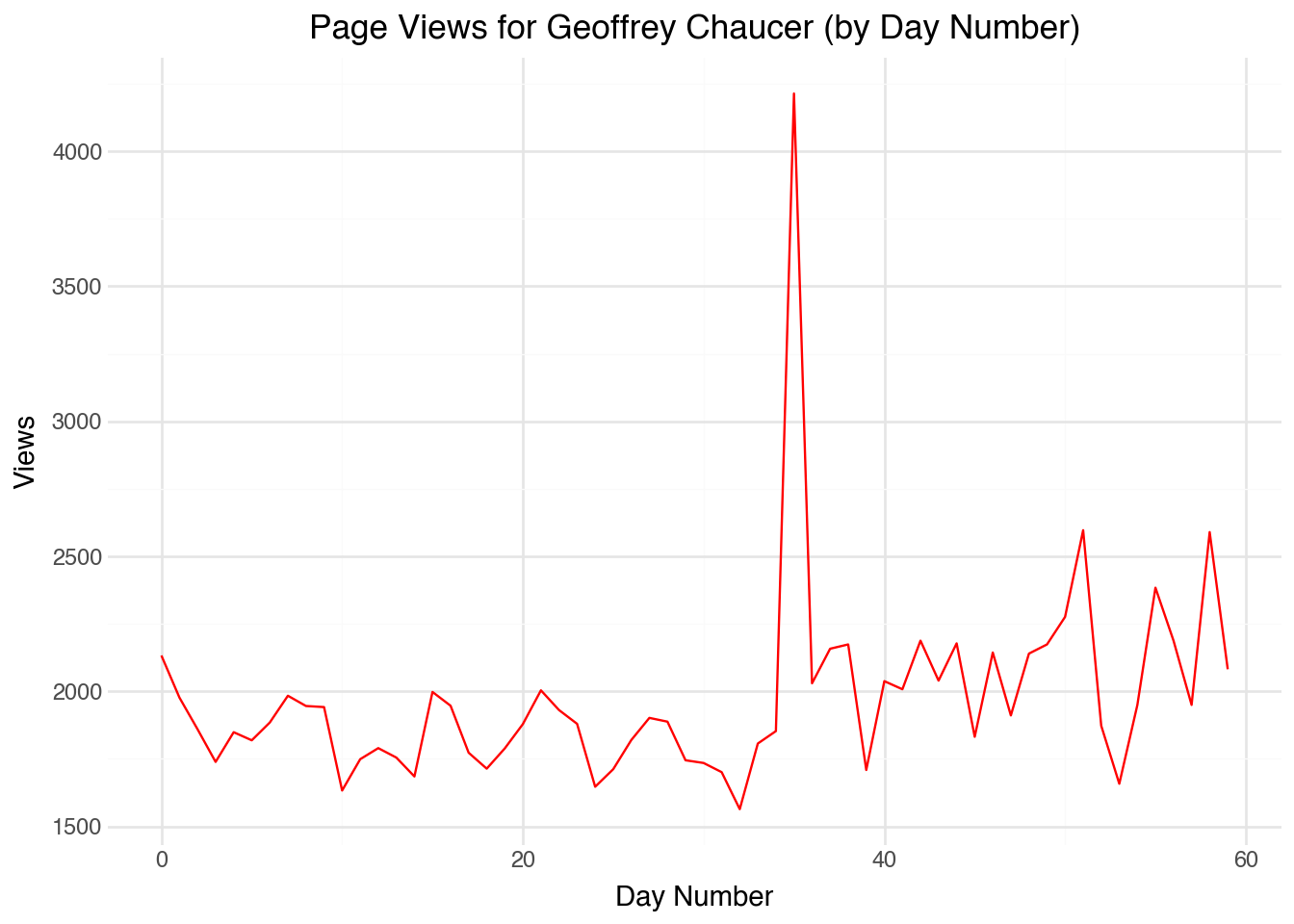
In this case, our starting plot is not a bad place to begin. The x-axis corresponds to the day number, and in many applications that may be exactly what we need. We can clearly see that the number of page views for Chaucer has a relatively stable count, possibly with some periodic swings over the course of the week. There is one day about two-thirds of the way through the plot in which the count spikes. Notice, though, that it is very hard to tell anything from the plot about exactly what days of the year are being represented. We cannot easily see which day has the spike in views, for example. Also, note that the correspondence between the row number and day only works because the data are uniformly sampled (one observation each day) and there is no missing data.
Another way to work with dates is to convert the data to a fractional year format. Here, the months and days are added to form a fractional day. A quick way to do this is to compute the following fractional year:
\[ year_{frac} = year + \frac{month - 1}{12} + \frac{day - 1}{12 \cdot 31}\]
We are subtracting one from the month and day so, for example, on a date such as 1 July 2020 (halfway through the year) we have the fractional year equal to 2020.5. We could make this even more exact by accounting for the fact that some months have fewer than 31 days, but as a first pass this works relatively well.
(
    page_views
    .filter(c.doc_id == "Geoffrey Chaucer")
    .with_columns(
        year_frac = c.year + (c.month - 1) / 12 + (c.day - 1) / (12 * 31)
    )
    .pipe(ggplot, aes("year_frac", "views"))
    + geom_line(color="red")
    + labs(
        title="Page Views for Geoffrey Chaucer (Fractional Year)",
        x="Fractional Year",
        y="Views"
    )
)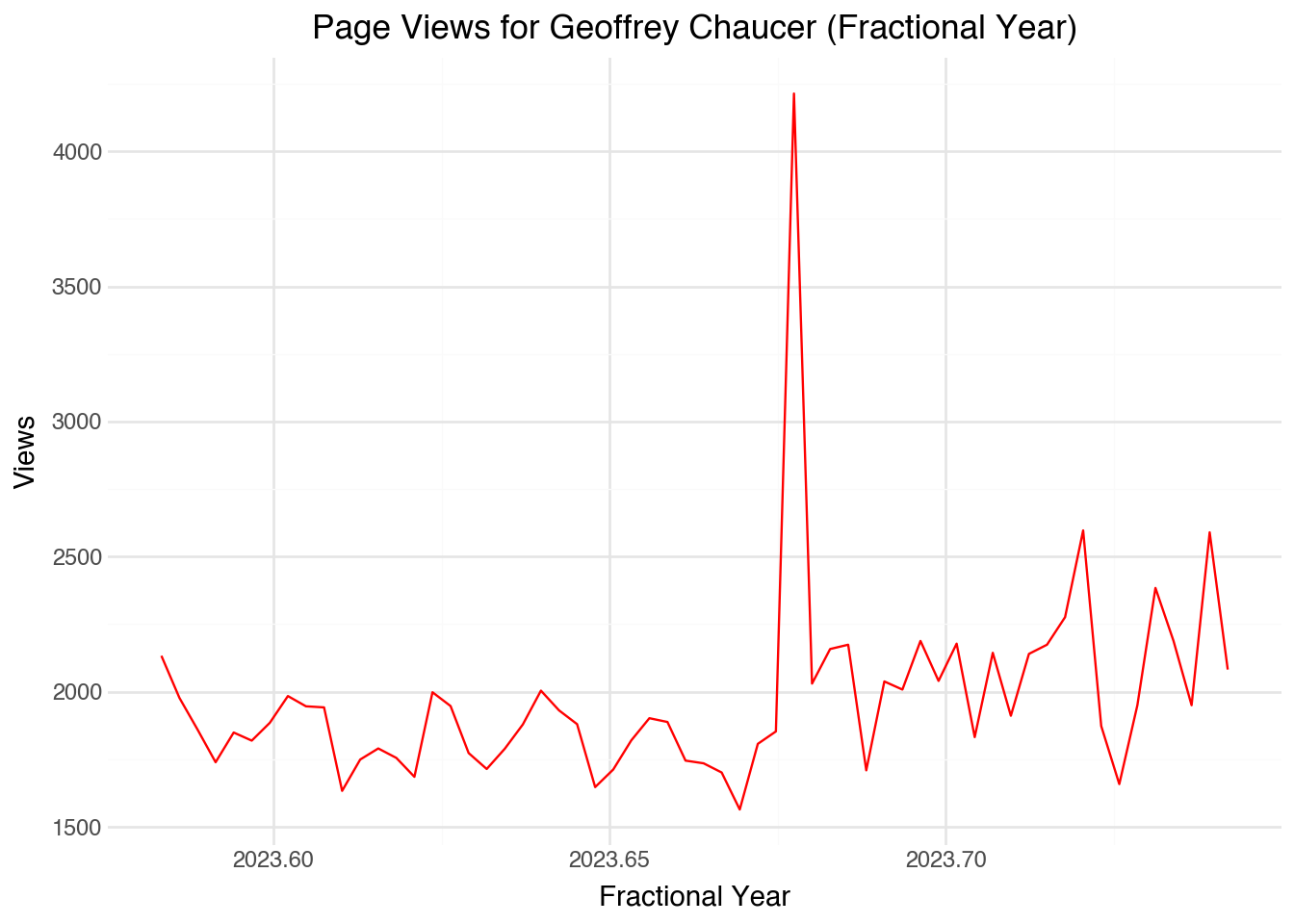
This revised visualization improves on several aspects of the original plot. For one thing, we can roughly see exactly what dates correspond to each data point. Also, the code will work fine regardless of whether the data are sorted, evenly distributed, or contain any missing values. As a downside, the axis labels take some explaining. We can extend the same approach to working with time data. For example, if we also had the (24-hour) time of our data points the formula would become:
\[ year_{frac} = year + \frac{month - 1}{12} + \frac{day - 1}{12 \cdot 31} + \frac{hour - 1}{24 \cdot 12 \cdot 31}\]
If we are only interested in the time since a specific event, say the start of an experiment, we can use the same approach but take the difference relative to a specific fractional year.
Fractional times have a number of important applications. Fractional times are convenient because they can represent an arbitrarily precise date or date-time with an ordinary number. This means that they can be used in other models and applications without any special treatment. They may require different model assumptions, but at least the code should work with minimal effort. This is a great way to explore our data. However, particularly when we want to create nice publishable visualizations, it can be useful to work with specific functions for manipulating dates and times.
17.4 Date Objects
Most of the variables that we have worked with so far are either strings or numbers. Dates are in some ways like numbers: they have a natural ordering, we can talk about the difference between two numbers, and it makes sense to color and plot them on a continuous scale. However, they do have some unique properties, particularly when we want to extract information such as the day of the week from a date, that require a unique data type. To create a date object in Polars, we can use the pl.date() function to construct a date from its components.
chaucer_with_dates = (
    page_views
    .filter(c.doc_id == "Geoffrey Chaucer")
    .with_columns(
        date = pl.date(c.year, c.month, c.day)
    )
)
chaucer_with_dates
shape: (60, 6)
| doc_id | year | month | day | views | date |
|---|---|---|---|---|---|
| str | i64 | i64 | i64 | i64 | date |
| "Geoffrey Chaucer" | 2023 | 8 | 1 | 2133 | 2023-08-01 |
| "Geoffrey Chaucer" | 2023 | 8 | 2 | 1977 | 2023-08-02 |
| "Geoffrey Chaucer" | 2023 | 8 | 3 | 1860 | 2023-08-03 |
| "Geoffrey Chaucer" | 2023 | 8 | 4 | 1739 | 2023-08-04 |
| "Geoffrey Chaucer" | 2023 | 8 | 5 | 1849 | 2023-08-05 |
| … | … | … | … | … | … |
| "Geoffrey Chaucer" | 2023 | 9 | 25 | 2384 | 2023-09-25 |
| "Geoffrey Chaucer" | 2023 | 9 | 26 | 2188 | 2023-09-26 |
| "Geoffrey Chaucer" | 2023 | 9 | 27 | 1950 | 2023-09-27 |
| "Geoffrey Chaucer" | 2023 | 9 | 28 | 2590 | 2023-09-28 |
| "Geoffrey Chaucer" | 2023 | 9 | 29 | 2082 | 2023-09-29 |
Notice that the new column has the special data type Date. If we build a visualization using a date object, plotnine is able to make helpful built-in choices about how to label the axis. For example, the following code will make a line plot that has nicely labeled values on the x-axis.
(
    chaucer_with_dates
    .pipe(ggplot, aes("date", "views"))
    + geom_line(color="red")
    + labs(
        title="Page Views for Geoffrey Chaucer",
        x="Date",
        y="Views"
    )
)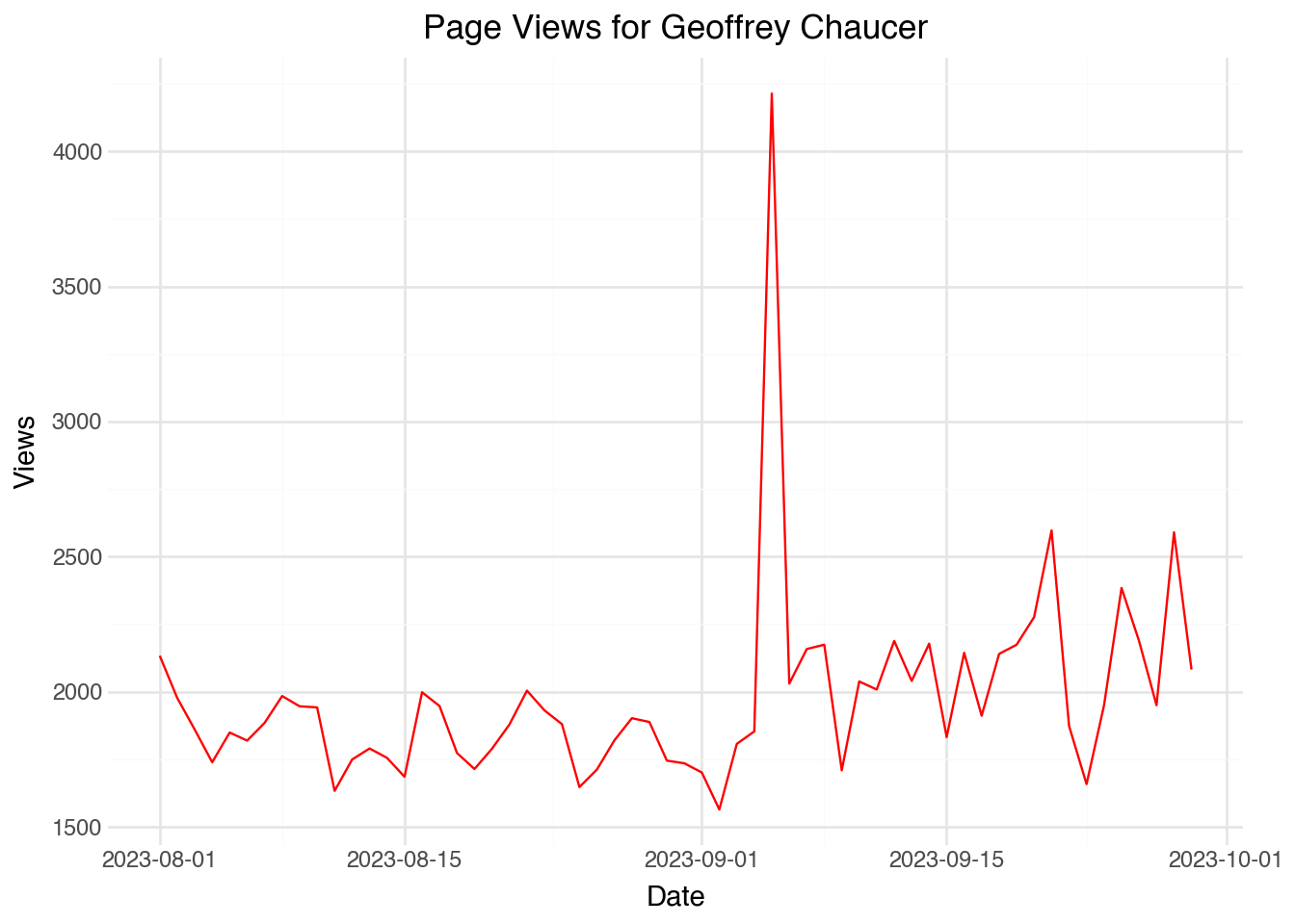
The output shows that the algorithm decided to label the dates appropriately. We can manually change the frequency of the labels using scale_x_date() and setting the date_breaks option. For example, the code below will display one label for each week:
(
    chaucer_with_dates
    .pipe(ggplot, aes("date", "views"))
    + geom_line(color="red")
    + scale_x_date(date_breaks="1 week", date_labels="%Y-%m-%d")
    + theme(axis_text_x=element_text(angle=45, hjust=1))
    + labs(
        title="Page Views for Geoffrey Chaucer (Weekly Labels)",
        x="Date",
        y="Views"
    )
)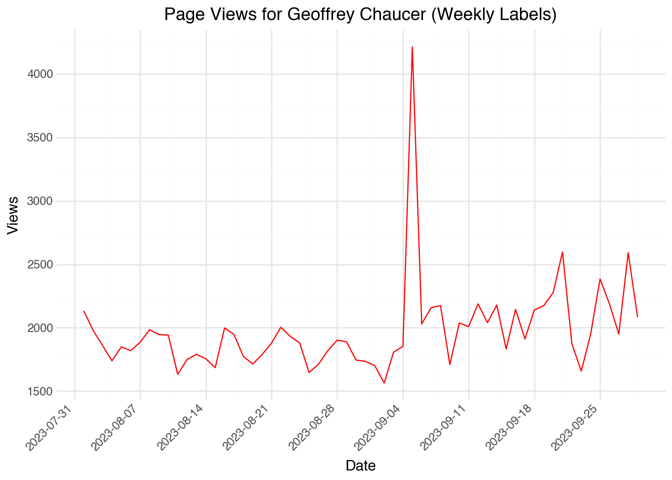
Once we have a date object, we can also extract useful information from it. For example, we can extract the weekday of the date using the .dt namespace in Polars. Here, we will compute the weekday and then calculate the average number of page views for each day of the week:
(
    chaucer_with_dates
    .with_columns(
        weekday = c.date.dt.weekday()
    )
    .group_by(c.weekday)
    .agg(
        views_avg = c.views.mean()
    )
    .sort(c.views_avg, descending=True)
)
shape: (7, 2)
| weekday | views_avg |
|---|---|
| i8 | f64 |
| 2 | 2273.111111 |
| 4 | 2098.555556 |
| 3 | 1988.111111 |
| 1 | 1975.75 |
| 7 | 1865.5 |
| 5 | 1828.222222 |
| 6 | 1762.375 |
Here we see the average number of page views by day of the week, where Monday is 1 and Sunday is 7. We can also use the date objects to filter the dataset. For example, we can filter the dataset to only include those dates after 15 January 2020, about two-thirds of the way through our dataset:
(
    chaucer_with_dates
    .filter(c.date > pl.date(2020, 1, 15))
)
shape: (60, 6)
| doc_id | year | month | day | views | date |
|---|---|---|---|---|---|
| str | i64 | i64 | i64 | i64 | date |
| "Geoffrey Chaucer" | 2023 | 8 | 1 | 2133 | 2023-08-01 |
| "Geoffrey Chaucer" | 2023 | 8 | 2 | 1977 | 2023-08-02 |
| "Geoffrey Chaucer" | 2023 | 8 | 3 | 1860 | 2023-08-03 |
| "Geoffrey Chaucer" | 2023 | 8 | 4 | 1739 | 2023-08-04 |
| "Geoffrey Chaucer" | 2023 | 8 | 5 | 1849 | 2023-08-05 |
| … | … | … | … | … | … |
| "Geoffrey Chaucer" | 2023 | 9 | 25 | 2384 | 2023-09-25 |
| "Geoffrey Chaucer" | 2023 | 9 | 26 | 2188 | 2023-09-26 |
| "Geoffrey Chaucer" | 2023 | 9 | 27 | 1950 | 2023-09-27 |
| "Geoffrey Chaucer" | 2023 | 9 | 28 | 2590 | 2023-09-28 |
| "Geoffrey Chaucer" | 2023 | 9 | 29 | 2082 | 2023-09-29 |
Note that we use the pl.date() function to create a date literal for comparison. Polars will also accept string representations of dates in ISO format for filtering.
Extracting date components
Polars provides many methods in the .dt namespace for extracting components from date and datetime objects. Common examples include .dt.year(), .dt.month(), .dt.day(), .dt.weekday(), .dt.ordinal_day() (day of year), and .dt.quarter(). These are useful for creating features for analysis or for grouping data by time periods.
17.5 Datetime Objects
The page_views dataset records the date of each observation. Sometimes we have data that describes the time of an event more specifically in terms of hours, minutes, and even possibly seconds. We will use the term datetime to describe an object that stores the precise time that an event occurs. The idea is that to describe the time that something happens we need to specify a date and a time. Later in the chapter, we will see an object that stores time without reference to a particular day. Whereas dates have a natural precision (a single day), we might desire to work with datetime objects of different levels of granularity. In some cases we might have just hours of the day and in others we might have access to records at the level of a millisecond such as data from radio and TV. In Polars, datetime objects are stored with microsecond precision by default, but we can regard the precision as whatever granularity we have given in our data for all practical purposes.
Datetime objects largely function the same as date objects. Let’s grab another dataset from Wikipedia that has precise timestamps. Below, we read in a dataset consisting of the last 500 edits made to each of the 75 British author pages in our collection.
page_revisions = (
    page_revisions
    .with_columns(
        datetime = c.datetime.str.to_datetime(time_zone="UTC")
    )
)
page_revisions
shape: (35_470, 5)
| doc_id | user | datetime | size | comment |
|---|---|---|---|---|
| str | str | datetime[μs, UTC] | i64 | str |
| "Marie de France" | "YurikBot" | 2006-07-06 23:24:54 UTC | 3061 | "robot Adding: [[it:Maria di F… |
| "Marie de France" | "YurikBot" | 2006-07-24 18:39:08 UTC | 3085 | "robot Adding: [[pt:Maria de F… |
| "Marie de France" | "Ccarroll" | 2006-09-10 13:36:44 UTC | 3085 | null |
| "Marie de France" | "63.231.20.88" | 2006-09-18 04:59:53 UTC | 3105 | null |
| "Marie de France" | "ExplicitImplicity" | 2006-09-23 22:27:20 UTC | 3104 | "i believe it is stupid to tran… |
| … | … | … | … | … |
| "Seamus Heaney" | "InternetArchiveBot" | 2023-09-21 04:51:45 UTC | 85491 | "Rescuing 1 sources and tagging… |
| "Seamus Heaney" | "81.110.56.233" | 2023-09-24 12:10:49 UTC | 85493 | null |
| "Seamus Heaney" | "149.50.162.177" | 2023-09-25 16:06:01 UTC | 85482 | "/* Death */" |
| "Seamus Heaney" | "--WikiUser1234945--" | 2023-09-25 16:06:11 UTC | 85493 | "Reverted edits by [[Special:Co… |
| "Seamus Heaney" | "BD2412" | 2023-09-27 02:39:46 UTC | 85493 | "/* 1957–1969 */Clean up spacin… |
Notice that each row has a record in the column datetime that provides a precise datetime object giving the second at which the page was modified. The data were stored using the ISO-8601 format (“YYYY-MM-DD HH:MM:SS”), which Polars can automatically parse with the .str.to_datetime() method.
Our page_revisions dataset includes several pieces of information about each of the edits. We have a username for the person who made the edit (recall that anyone can edit a Wikipedia page), the size in bytes of the page after the edit was made, and a short comment describing what was done in the change. Looking at the page size over time shows when large additions and deletions were made to each record. The code below yields a temporal visualization:
selected_authors = ["Geoffrey Chaucer", "Emily Brontë"]
(
    page_revisions
    .filter(c.doc_id.is_in(selected_authors))
    .pipe(ggplot, aes("datetime", "size", color="doc_id"))
    + geom_line()
    + scale_color_manual(values=["red", "blue"])
    + labs(
        title="Wikipedia Page Size Over Time",
        x="Date",
        y="Page Size (bytes)",
        color="Author"
    )
)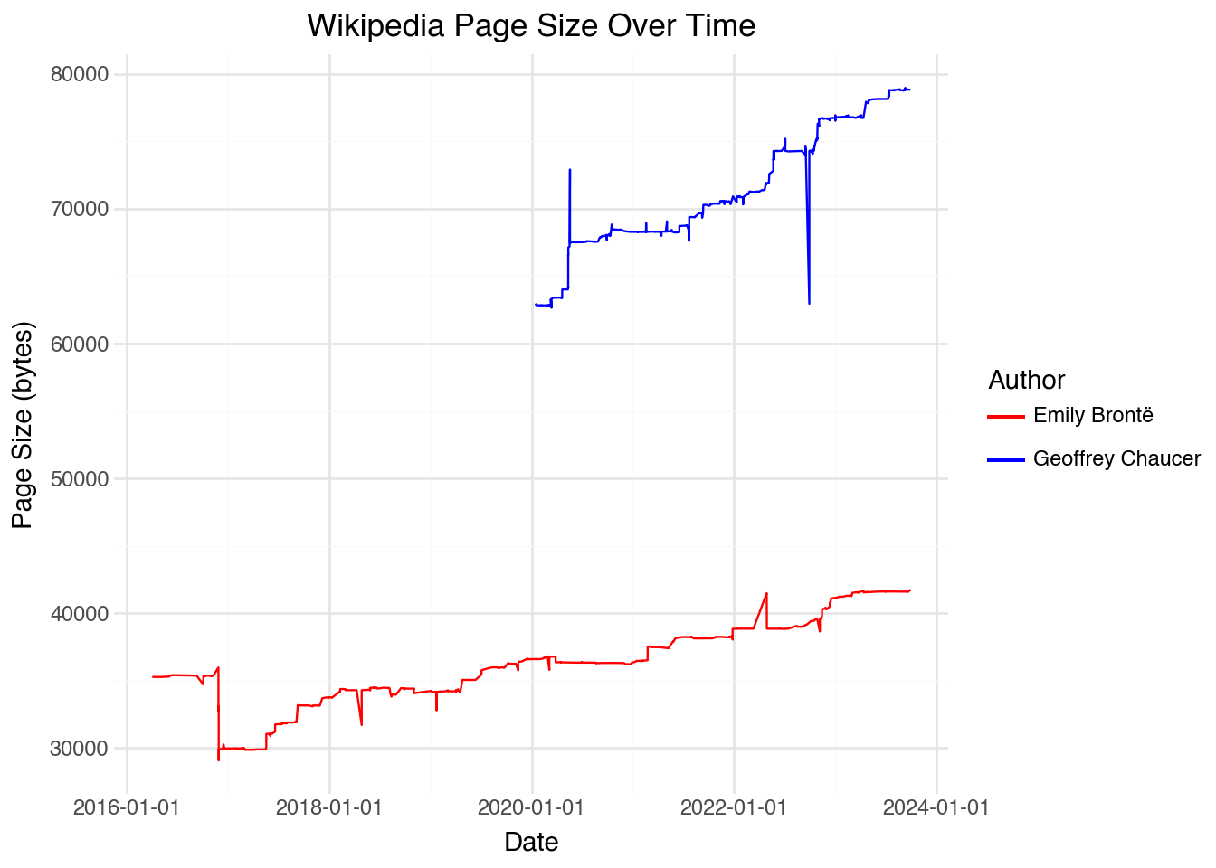
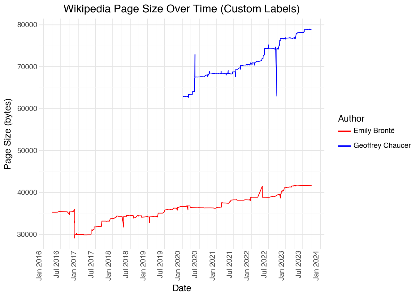
Looking at the plot, we can see that there are a few very large edits (both deletions and additions), likely consisting of large sections added and subtracted from the page. If we want to visualize when these large changes occurred, it would be useful to include a more granular set of labels on the x-axis. We can do this using scale_x_datetime() with custom formatting:
(
    page_revisions
    .filter(c.doc_id.is_in(selected_authors))
    .pipe(ggplot, aes("datetime", "size", color="doc_id"))
    + geom_line()
    + scale_color_manual(values=["red", "blue"])
    + scale_x_datetime(date_breaks="6 months", date_labels="%b %Y")
    + theme(axis_text_x=element_text(angle=90, hjust=1))
    + labs(
        title="Wikipedia Page Size Over Time (Custom Labels)",
        x="Date",
        y="Page Size (bytes)",
        color="Author"
    )
)
We can also filter our dataset by a particular range of dates or times. This is useful to zoom into a specific region of our data to investigate patterns that may be otherwise lost. For example, if we wanted to see all of the page sizes for two authors from 2021 onward:
(
    page_revisions
    .filter(c.doc_id.is_in(selected_authors))
    .filter(c.datetime > pl.datetime(2021, 1, 1, time_zone="UTC"))
)
shape: (506, 5)
| doc_id | user | datetime | size | comment |
|---|---|---|---|---|
| str | str | datetime[μs, UTC] | i64 | str |
| "Geoffrey Chaucer" | "86.31.15.58" | 2021-01-18 09:42:33 UTC | 68291 | "/* Origin */" |
| "Geoffrey Chaucer" | "86.31.15.58" | 2021-01-18 09:43:16 UTC | 68288 | "/* Taco Bell */" |
| "Geoffrey Chaucer" | "88.108.207.22" | 2021-01-18 11:15:33 UTC | 68284 | "/* Career */" |
| "Geoffrey Chaucer" | "Pahunkat" | 2021-01-18 11:16:09 UTC | 68288 | "Rollback edit(s) by [[Special:… |
| "Geoffrey Chaucer" | "88.108.207.22" | 2021-01-18 11:16:40 UTC | 68293 | "/* Origin */" |
| … | … | … | … | … |
| "Emily Brontë" | "HeyElliott" | 2023-09-16 20:05:37 UTC | 41598 | "[[WP:LQ]]" |
| "Emily Brontë" | "Qwerfjkl (bot)" | 2023-09-21 16:34:46 UTC | 41586 | "Converting Gutenberg author ID… |
| "Emily Brontë" | "Ficaia" | 2023-09-27 12:47:22 UTC | 41717 | null |
| "Emily Brontë" | "Keith D" | 2023-09-27 20:36:18 UTC | 41688 | "Remove namespace | Replaced cu… |
| "Emily Brontë" | "Keith D" | 2023-09-27 20:39:51 UTC | 41693 | "/* Adulthood */ Cite fix" |
Notice that the filter includes data from 2021, even though we use a strictly greater than condition. The reason for this is that pl.datetime(2021, 1, 1) is interpreted as the exact time corresponding to 1 January 2021 at 00:00. Any record that comes at any other time during the year of 2021 will be included in the filter.
17.6 Language and Time Zones
So far, we have primarily worked with numeric summaries of the date and datetime objects. In the previous sections, notice that our example of working with the days of the week used numeric values (1-7) rather than names. Polars provides methods to extract string names for weekdays and months, though the output depends on your system locale. Below, for example, we extract various datetime components:
(
    page_revisions
    .head(10)
    .with_columns(
        weekday_num = c.datetime.dt.weekday(),
        month_num = c.datetime.dt.month(),
        hour = c.datetime.dt.hour(),
        date_only = c.datetime.dt.date()
    )
    .select(c.datetime, c.weekday_num, c.month_num, c.hour, c.date_only)
)
shape: (10, 5)
| datetime | weekday_num | month_num | hour | date_only |
|---|---|---|---|---|
| datetime[μs, UTC] | i8 | i8 | i8 | date |
| 2006-07-06 23:24:54 UTC | 4 | 7 | 23 | 2006-07-06 |
| 2006-07-24 18:39:08 UTC | 1 | 7 | 18 | 2006-07-24 |
| 2006-09-10 13:36:44 UTC | 7 | 9 | 13 | 2006-09-10 |
| 2006-09-18 04:59:53 UTC | 1 | 9 | 4 | 2006-09-18 |
| 2006-09-23 22:27:20 UTC | 6 | 9 | 22 | 2006-09-23 |
| 2006-09-23 22:31:03 UTC | 6 | 9 | 22 | 2006-09-23 |
| 2006-10-03 18:18:09 UTC | 2 | 10 | 18 | 2006-10-03 |
| 2006-10-03 18:19:32 UTC | 2 | 10 | 18 | 2006-10-03 |
| 2006-10-10 18:48:26 UTC | 2 | 10 | 18 | 2006-10-10 |
| 2006-10-11 05:29:32 UTC | 3 | 10 | 5 | 2006-10-11 |
Weekday and month names
If you need weekday or month names as strings, you can create a mapping from the numeric values. For example, you could use pl.when() chains or join with a lookup table. The numeric representation is often more convenient for analysis and avoids locale-dependent issues.
Another regional issue that arises when working with dates and times are time zones. While seemingly not too difficult a concept, getting time zones to work correctly with complex datasets can be incredibly complicated. A wide range of programming bugs have been attributed to all sorts of edge-cases surrounding the processing of time zones.
All times stored in Polars can be timezone-aware or timezone-naive. By default, times are stored as timezone-naive (no timezone information). The data can be localized to a specific timezone using the .dt.replace_time_zone() method, and converted between time zones using .dt.convert_time_zone(). All of the times recorded in the dataset page_revisions are given in UTC. This is not surprising; most technical sources with a global focus will use this convention.
We can convert between time zones using Polars datetime methods. Since we parsed our data with time_zone="UTC", the datetime column is already timezone-aware. We can convert to another timezone using .dt.convert_time_zone(). Let’s convert our UTC times to New York time:
(
    page_revisions
    .head(10)
    .with_columns(
        datetime_utc = c.datetime,
        datetime_nyc = c.datetime.dt.convert_time_zone("America/New_York")
    )
    .with_columns(
        hour_utc = c.datetime_utc.dt.hour(),
        hour_nyc = c.datetime_nyc.dt.hour()
    )
    .select(c.datetime_utc, c.datetime_nyc, c.hour_utc, c.hour_nyc)
)
shape: (10, 4)
| datetime_utc | datetime_nyc | hour_utc | hour_nyc |
|---|---|---|---|
| datetime[μs, UTC] | datetime[μs, America/New_York] | i8 | i8 |
| 2006-07-06 23:24:54 UTC | 2006-07-06 19:24:54 EDT | 23 | 19 |
| 2006-07-24 18:39:08 UTC | 2006-07-24 14:39:08 EDT | 18 | 14 |
| 2006-09-10 13:36:44 UTC | 2006-09-10 09:36:44 EDT | 13 | 9 |
| 2006-09-18 04:59:53 UTC | 2006-09-18 00:59:53 EDT | 4 | 0 |
| 2006-09-23 22:27:20 UTC | 2006-09-23 18:27:20 EDT | 22 | 18 |
| 2006-09-23 22:31:03 UTC | 2006-09-23 18:31:03 EDT | 22 | 18 |
| 2006-10-03 18:18:09 UTC | 2006-10-03 14:18:09 EDT | 18 | 14 |
| 2006-10-03 18:19:32 UTC | 2006-10-03 14:19:32 EDT | 18 | 14 |
| 2006-10-10 18:48:26 UTC | 2006-10-10 14:48:26 EDT | 18 | 14 |
| 2006-10-11 05:29:32 UTC | 2006-10-11 01:29:32 EDT | 5 | 1 |
We can use the timezone information to display data in a useful way to a local audience. For example, the code below displays the frequency of updates as a function of the hour of the day in New York City:
hourly_edits = (
    page_revisions
    .with_columns(
        datetime_nyc = c.datetime.dt.convert_time_zone("America/New_York")
    )
    .with_columns(
        hour_nyc = c.datetime_nyc.dt.hour()
    )
    .group_by(c.hour_nyc)
    .agg(
        count = pl.len()
    )
    .sort(c.hour_nyc)
)

(
    hourly_edits
    .pipe(ggplot, aes("hour_nyc", "count"))
    + geom_col()
    + labs(
        title="Wikipedia Edits by Hour (New York Time)",
        x="Hour of Day",
        y="Number of Edits"
    )
)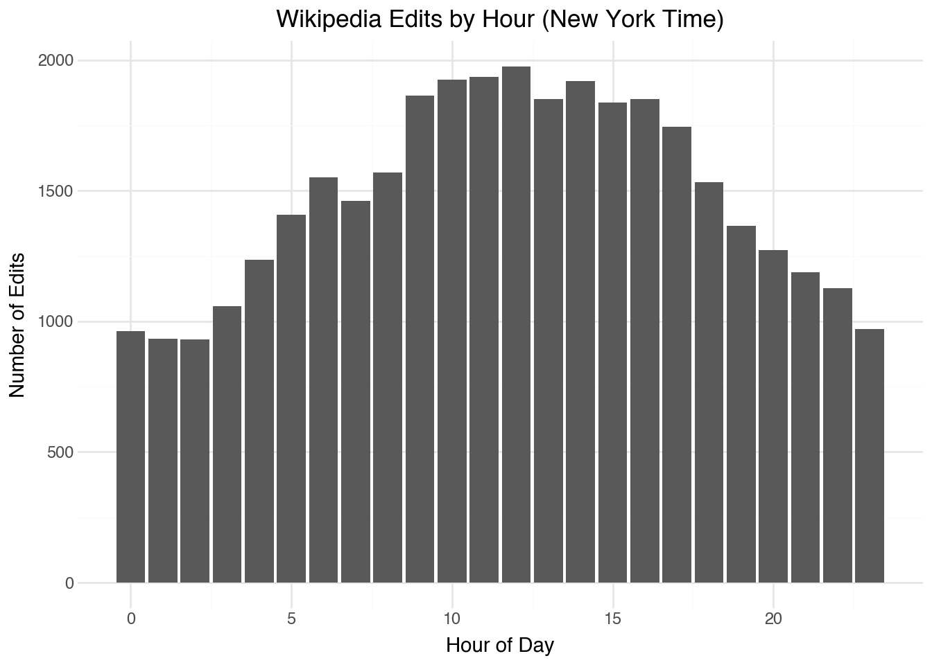
While certainly many editors are living in other English-speaking cities (London, Los Angeles, or Mumbai), it is generally easier for people to do the mental math for what times correspond relative to their own time zone than relative to UTC.
17.7 Truncating Dates Data
We have shown above how to create date and datetime objects using Polars functions. Also, we have seen how to extract the components from date and datetime objects with the .dt namespace. There are a variety of other functions that help us create and manipulate these temporal objects. While we will not give an entire list of all the available functions in Polars datetime functionality, let’s look at a few of the most useful and representative examples for converting between different ways of representing information about time.
The page_revisions dataset has revisions recorded with the precision of a second. This is likely overly granular for many applications; it might be better to have the data in a format that is only at the level of an hour, for example. We can truncate any date or datetime object by using the .dt.truncate() method along with a specific duration. Setting the duration to “1h” (one hour), for example, will remove all of the minutes and seconds from the time:
(
    page_revisions
    .head(10)
    .with_columns(
        datetime_hour = c.datetime.dt.truncate("1h"),
        datetime_day = c.datetime.dt.truncate("1d")
    )
    .select(c.datetime, c.datetime_hour, c.datetime_day)
)
shape: (10, 3)
| datetime | datetime_hour | datetime_day |
|---|---|---|
| datetime[μs, UTC] | datetime[μs, UTC] | datetime[μs, UTC] |
| 2006-07-06 23:24:54 UTC | 2006-07-06 23:00:00 UTC | 2006-07-06 00:00:00 UTC |
| 2006-07-24 18:39:08 UTC | 2006-07-24 18:00:00 UTC | 2006-07-24 00:00:00 UTC |
| 2006-09-10 13:36:44 UTC | 2006-09-10 13:00:00 UTC | 2006-09-10 00:00:00 UTC |
| 2006-09-18 04:59:53 UTC | 2006-09-18 04:00:00 UTC | 2006-09-18 00:00:00 UTC |
| 2006-09-23 22:27:20 UTC | 2006-09-23 22:00:00 UTC | 2006-09-23 00:00:00 UTC |
| 2006-09-23 22:31:03 UTC | 2006-09-23 22:00:00 UTC | 2006-09-23 00:00:00 UTC |
| 2006-10-03 18:18:09 UTC | 2006-10-03 18:00:00 UTC | 2006-10-03 00:00:00 UTC |
| 2006-10-03 18:19:32 UTC | 2006-10-03 18:00:00 UTC | 2006-10-03 00:00:00 UTC |
| 2006-10-10 18:48:26 UTC | 2006-10-10 18:00:00 UTC | 2006-10-10 00:00:00 UTC |
| 2006-10-11 05:29:32 UTC | 2006-10-11 05:00:00 UTC | 2006-10-11 00:00:00 UTC |
The benefit of using the .dt.truncate() method is that we could then group, join, or summarize the data in a way that treats each value of datetime the same as long as they occur during the same hour. There is also a .dt.round() method for rounding the datetime object to the nearest desired unit. In the special case in which we want to extract just the date part of a datetime, we can use the .dt.date() method. The code below illustrates this process, as well as showing how reducing the temporal granularity can be a useful first step before grouping and summarizing:
(
    page_revisions
    .with_columns(
        date = c.datetime.dt.date()
    )
    .group_by(c.date)
    .agg(
        count = pl.len()
    )
    .sort(c.date, descending=True)
)
shape: (4_831, 2)
| date | count |
|---|---|
| date | u32 |
| 2023-09-30 | 10 |
| 2023-09-29 | 11 |
| 2023-09-28 | 9 |
| 2023-09-27 | 14 |
| 2023-09-26 | 12 |
| … | … |
| 2003-02-01 | 1 |
| 2003-01-29 | 2 |
| 2003-01-14 | 1 |
| 2003-01-04 | 1 |
| 2002-10-26 | 1 |
Above, we effectively remove the time component of the datetime object and treat the variable as having only a date element. Occasionally, we might want to do the opposite: considering only the time component of a datetime object without worrying about the specific date. For example, we might want to summarize the number of edits that are made based on the time of the day. We can do this by extracting the hour component:
(
    page_revisions
    .with_columns(
        hour = c.datetime.dt.hour()
    )
    .group_by(c.hour)
    .agg(
        count = pl.len()
    )
    .sort(c.hour)
)
shape: (24, 2)
| hour | count |
|---|---|
| i8 | u32 |
| 0 | 1316 |
| 1 | 1229 |
| 2 | 1149 |
| 3 | 1010 |
| 4 | 982 |
| … | … |
| 19 | 1837 |
| 20 | 1838 |
| 21 | 1797 |
| 22 | 1675 |
| 23 | 1349 |
This creates a variable that stores the hour without any date information, which is useful for analyzing patterns that repeat daily.
17.8 Window Functions
At the start of this chapter, we considered time series to be a sequence of events without too much focus on the specific dates and times. This viewpoint can be a useful construct when we want to look at changes over time. For example, we have the overall size of each Wikipedia page after an edit. A measurement that would be useful is the difference in page size made by an edit. To add a variable to a dataset, we usually use the .with_columns() method, and that will again work here. However, in this case we need to reference values that come before or after a certain value. This requires the use of window functions.
A window function transforms a variable in a dataset into a new variable with the same length in a way that takes into account the entire ordering of the data. Two examples of window functions that are useful when working with time series data are .shift() with positive and negative values, which give access to rows preceding or following a row, respectively. Let’s apply this to our dataset of page revisions to get the previous and next values of the page size variable.
(
    page_revisions
    .with_columns(
        size_last = c.size.shift(1),
        size_next = c.size.shift(-1)
    )
    .select(c.doc_id, c.datetime, c.size, c.size_last, c.size_next)
)
shape: (35_470, 5)
| doc_id | datetime | size | size_last | size_next |
|---|---|---|---|---|
| str | datetime[μs, UTC] | i64 | i64 | i64 |
| "Marie de France" | 2006-07-06 23:24:54 UTC | 3061 | null | 3085 |
| "Marie de France" | 2006-07-24 18:39:08 UTC | 3085 | 3061 | 3085 |
| "Marie de France" | 2006-09-10 13:36:44 UTC | 3085 | 3085 | 3105 |
| "Marie de France" | 2006-09-18 04:59:53 UTC | 3105 | 3085 | 3104 |
| "Marie de France" | 2006-09-23 22:27:20 UTC | 3104 | 3105 | 3132 |
| … | … | … | … | … |
| "Seamus Heaney" | 2023-09-21 04:51:45 UTC | 85491 | 85341 | 85493 |
| "Seamus Heaney" | 2023-09-24 12:10:49 UTC | 85493 | 85491 | 85482 |
| "Seamus Heaney" | 2023-09-25 16:06:01 UTC | 85482 | 85493 | 85493 |
| "Seamus Heaney" | 2023-09-25 16:06:11 UTC | 85493 | 85482 | 85493 |
| "Seamus Heaney" | 2023-09-27 02:39:46 UTC | 85493 | 85493 | null |
Notice that the first value of size_last is missing because there is no last value for the first item in our data. Similarly, the variable size_next will have a missing value at the end of the dataset. As written above, the code incorrectly crosses the time points at the boundary of each page. That is, for the first row of the second page (Geoffrey Chaucer) it thinks that the size of the last page is the size of the final page of the Marie de France record. To fix this, we can use the .over() method to apply the window function within groups. Window functions respect the grouping of the data:
(
    page_revisions
    .sort(c.doc_id, c.datetime)
    .with_columns(
        size_last = c.size.shift(1).over(c.doc_id),
        size_next = c.size.shift(-1).over(c.doc_id)
    )
    .select(c.doc_id, c.datetime, c.size, c.size_last, c.size_next)
    .slice(495, 10)
)
shape: (10, 5)
| doc_id | datetime | size | size_last | size_next |
|---|---|---|---|---|
| str | datetime[μs, UTC] | i64 | i64 | i64 |
| "A. A. Milne" | 2023-08-05 20:59:54 UTC | 44019 | 43990 | 44038 |
| "A. A. Milne" | 2023-08-18 09:26:21 UTC | 44038 | 44019 | 44044 |
| "A. A. Milne" | 2023-08-21 22:05:31 UTC | 44044 | 44038 | 44045 |
| "A. A. Milne" | 2023-08-21 22:07:46 UTC | 44045 | 44044 | 44077 |
| "A. A. Milne" | 2023-08-31 20:41:54 UTC | 44077 | 44045 | null |
| "Alexander Pope" | 2016-04-17 04:03:45 UTC | 31345 | null | 31531 |
| "Alexander Pope" | 2016-05-05 22:17:54 UTC | 31531 | 31345 | 31532 |
| "Alexander Pope" | 2016-05-05 22:24:29 UTC | 31532 | 31531 | 31585 |
| "Alexander Pope" | 2016-05-07 19:05:49 UTC | 31585 | 31532 | 31614 |
| "Alexander Pope" | 2016-05-09 17:22:21 UTC | 31614 | 31585 | 31585 |
Notice that now, correctly, the dataset has a missing size_next for the final Marie de France record and a missing size_last for the first Geoffrey Chaucer record. Now, let’s use this to compute the change in the page sizes for each of the revisions:
(
    page_revisions
    .sort(c.doc_id, c.datetime)
    .with_columns(
        size_diff = c.size - c.size.shift(1).over(c.doc_id)
    )
    .select(c.doc_id, c.datetime, c.size, c.size_diff)
)
shape: (35_470, 4)
| doc_id | datetime | size | size_diff |
|---|---|---|---|
| str | datetime[μs, UTC] | i64 | i64 |
| "A. A. Milne" | 2015-09-04 16:30:26 UTC | 30702 | null |
| "A. A. Milne" | 2015-09-22 14:51:08 UTC | 30400 | -302 |
| "A. A. Milne" | 2015-11-07 10:23:31 UTC | 30389 | -11 |
| "A. A. Milne" | 2015-11-08 00:48:23 UTC | 30397 | 8 |
| "A. A. Milne" | 2015-11-16 03:12:19 UTC | 30427 | 30 |
| … | … | … | … |
| "William Wordsworth" | 2023-09-25 11:19:40 UTC | 41466 | 0 |
| "William Wordsworth" | 2023-09-27 15:10:27 UTC | 41464 | -2 |
| "William Wordsworth" | 2023-09-27 15:11:44 UTC | 41466 | 2 |
| "William Wordsworth" | 2023-09-27 15:13:48 UTC | 41467 | 1 |
| "William Wordsworth" | 2023-09-27 15:18:10 UTC | 41466 | -1 |
In the above output, we can see the changes in page sizes. If we wanted to find reversions in the dataset, we could apply the .shift() function several times. As an alternative, we can also give a parameter to .shift() to indicate that we want to go back (or forward) more than one row. Let’s put this together to indicate which commits seem to be a reversion (the page size exactly matches the page size from two commits prior) as well as the overall size of the reversion:
(
    page_revisions
    .sort(c.doc_id, c.datetime)
    .with_columns(
        size_diff = c.size - c.size.shift(1).over(c.doc_id),
        size_two_back = c.size.shift(2).over(c.doc_id),
        is_reversion = c.size == c.size.shift(2).over(c.doc_id)
    )
    .filter(c.is_reversion)
    .select(c.doc_id, c.datetime, c.size_diff, c.is_reversion)
)
shape: (4_927, 4)
| doc_id | datetime | size_diff | is_reversion |
|---|---|---|---|
| str | datetime[μs, UTC] | i64 | bool |
| "A. A. Milne" | 2015-12-17 18:13:11 UTC | -6 | true |
| "A. A. Milne" | 2016-01-07 18:55:26 UTC | 30407 | true |
| "A. A. Milne" | 2016-04-14 17:38:45 UTC | 36 | true |
| "A. A. Milne" | 2016-04-17 15:06:58 UTC | -77 | true |
| "A. A. Milne" | 2016-04-27 20:04:19 UTC | -1 | true |
| … | … | … | … |
| "William Wordsworth" | 2023-09-18 06:35:43 UTC | -1 | true |
| "William Wordsworth" | 2023-09-24 14:54:33 UTC | 8 | true |
| "William Wordsworth" | 2023-09-25 11:19:40 UTC | 0 | true |
| "William Wordsworth" | 2023-09-27 15:11:44 UTC | 2 | true |
| "William Wordsworth" | 2023-09-27 15:18:10 UTC | -1 | true |
These reversions can be studied to see the nature of the Wikipedia editing process. For example, how long do these reversions tend to take? Are certain pages more likely to undergo reversions? Do these take place during a certain time of the day? These are all questions that we should now be able to address using this dataset and the tools described above.
Additional window functions
Polars provides many other window functions beyond .shift(). Common examples include .cum_sum() for cumulative sums, .rolling_mean() for moving averages, .rank() for ranking values, and .diff() which computes the difference between consecutive values (equivalent to x - x.shift(1)). All of these can be combined with .over() to apply within groups.
17.9 Range Joins
We will finish this chapter by looking at range joins, which allow for combining datasets based on inequalities between keys contained in two different datasets. Range joins are functionality that can greatly simplify some operations that arise when working with temporal data. Recall that all of the join functions that we saw in Chapter 4 work by finding a correspondence where keys from one dataset equal the values of keys in another dataset. In some cases it happens that we want to join two tables on inequalities rather than exact values.
Take, for example, the metadata table for the 75 authors in our Wikipedia collection. Recall that this dataset contains the years that each author was born and the years each author died. What if we wanted to make a dataset by joining the metadata to itself, matching each author with other authors that would have been alive in overlapping years? We can do this using Polars’ .join_where() method:
(
    meta
    .join_where(
        meta,
        (c.born <= c.born_right) & (c.died > c.born_right) & (c.doc_id != c.doc_id_right)
    )
    .select(c.doc_id, c.doc_id_right, c.born, c.died, c.born_right, c.died_right)
)
shape: (693, 6)
| doc_id | doc_id_right | born | died | born_right | died_right |
|---|---|---|---|---|---|
| str | str | i64 | i64 | i64 | i64 |
| "Stephen Spender" | "Seamus Heaney" | 1909 | 1995 | 1939 | 1939 |
| "Daphne du Maurier" | "Seamus Heaney" | 1907 | 1989 | 1939 | 1939 |
| "Daphne du Maurier" | "Stephen Spender" | 1907 | 1989 | 1909 | 1995 |
| "Daphne du Maurier" | "W. H. Auden" | 1907 | 1989 | 1907 | 1973 |
| "Daphne du Maurier" | "Louis MacNeice" | 1907 | 1989 | 1907 | 1963 |
| … | … | … | … | … | … |
| "William Langland" | "Geoffrey Chaucer" | 1332 | 1386 | 1343 | 1400 |
| "John Gower" | "Thomas Malory" | 1330 | 1408 | 1405 | 1471 |
| "John Gower" | "Margery Kempe" | 1330 | 1408 | 1373 | 1438 |
| "John Gower" | "Geoffrey Chaucer" | 1330 | 1408 | 1343 | 1400 |
| "John Gower" | "William Langland" | 1330 | 1408 | 1332 | 1386 |
The .join_where() method takes one or more expressions to specify which pairs of rows to keep in the joined dataset. To refer to columns in the second (right) dataset that share the same name, use the _right suffix. In the example above, we find all pairs where the first author’s lifespan overlaps with the second author’s birth, excluding self-matches.
The resulting dataset would make an interesting type of network, showing temporal overlap of authors in the dataset. We will investigate this in the following chapter.
Performance of conditional joins
The .join_where() method can be slow because it needs to check every combination of rows in the two datasets. For large datasets, consider whether you can use .join_asof() instead, which is optimized for nearest-value matching and requires the data to be sorted. The .join_asof() method is particularly useful when you want to match each row to the nearest (or nearest preceding/following) value in another dataset.
17.10 Temporal Durations
Sometimes we want to work not with specific dates or times, but with durations—the amount of time between two events. Polars represents durations with the Duration data type. We can compute durations by subtracting one datetime from another, or by using the pl.duration() function to create specific intervals.
(
    page_revisions
    .sort(c.doc_id, c.datetime)
    .with_columns(
        time_since_last = c.datetime - c.datetime.shift(1).over(c.doc_id)
    )
    .select(c.doc_id, c.datetime, c.time_since_last)
    .drop_nulls()
)
shape: (35_395, 3)
| doc_id | datetime | time_since_last |
|---|---|---|
| str | datetime[μs, UTC] | duration[μs] |
| "A. A. Milne" | 2015-09-22 14:51:08 UTC | 17d 22h 20m 42s |
| "A. A. Milne" | 2015-11-07 10:23:31 UTC | 45d 19h 32m 23s |
| "A. A. Milne" | 2015-11-08 00:48:23 UTC | 14h 24m 52s |
| "A. A. Milne" | 2015-11-16 03:12:19 UTC | 8d 2h 23m 56s |
| "A. A. Milne" | 2015-11-17 07:52:16 UTC | 1d 4h 39m 57s |
| … | … | … |
| "William Wordsworth" | 2023-09-25 11:19:40 UTC | 1h 17m |
| "William Wordsworth" | 2023-09-27 15:10:27 UTC | 2d 3h 50m 47s |
| "William Wordsworth" | 2023-09-27 15:11:44 UTC | 1m 17s |
| "William Wordsworth" | 2023-09-27 15:13:48 UTC | 2m 4s |
| "William Wordsworth" | 2023-09-27 15:18:10 UTC | 4m 22s |
The resulting duration can be converted to various units using methods like .dt.total_days(), .dt.total_hours(), .dt.total_minutes(), or .dt.total_seconds(). This is useful for analyzing how frequently events occur or how long processes take.
(
    page_revisions
    .sort(c.doc_id, c.datetime)
    .with_columns(
        time_since_last = c.datetime - c.datetime.shift(1).over(c.doc_id)
    )
    .with_columns(
        days_since_last = c.time_since_last.dt.total_days()
    )
    .select(c.doc_id, c.datetime, c.days_since_last)
    .drop_nulls()
    .group_by(c.doc_id)
    .agg(
        avg_days_between_edits = c.days_since_last.mean()
    )
    .sort(c.avg_days_between_edits)
)
shape: (75, 2)
| doc_id | avg_days_between_edits |
|---|---|
| str | f64 |
| "George Orwell" | 1.138277 |
| "James Joyce" | 1.224449 |
| "Oscar Wilde" | 1.58517 |
| "Thomas More" | 1.791583 |
| "Percy Bysshe Shelley" | 1.815631 |
| … | … |
| "John Gower" | 24.467105 |
| "Edward Upward" | 27.0 |
| "Katherine Philipps" | 31.182692 |
| "Rex Warner" | 39.488506 |
| "Charlotte Smith" | 168.222222 |
This shows us which Wikipedia pages are edited most frequently (smallest average days between edits) and which are edited less often.
17.11 Summary
In this chapter, we explored techniques for working with temporal data in Polars. We learned how to create date and datetime objects from their components, extract useful information from them, and visualize temporal patterns. We saw how to work with time zones and how to truncate temporal data to different levels of granularity. Window functions allowed us to compare values across time within groups, and range joins provided a way to combine datasets based on temporal overlap. These tools are essential for any analysis involving time-based data.