import numpy as np
import polars as pl

from funs import *
from plotnine import *
from polars import col as c
theme_set(theme_minimal())

metro = pl.read_csv("data/acs_cbsa.csv")16 Spatial Data
16.1 Setup
Load all of the modules and datasets needed for the chapter.
16.2 Introduction
Every piece of data we have worked with so far in this book has existed in an abstract space defined only by the relationships between variables. A country’s GDP, a patient’s blood pressure, or a product’s sales figures are all numbers that live in a purely numerical realm. But much of the world’s most valuable data is inherently tied to physical locations on Earth. Where did this crime occur? Which neighborhoods have the highest rates of asthma? How far is the nearest hospital from each school? These questions require a fundamentally different approach to data analysis, one that treats location not as just another variable but as a geometric object with shape, area, and spatial relationships to other objects.
Spatial data analysis bridges the gap between traditional tabular data and the physical world. At its core, spatial data associates each observation with a geometry: a mathematical representation of a location or region on Earth’s surface. A geometry might be as simple as a single point (the location of a coffee shop) or as complex as a polygon with thousands of vertices (the boundary of a congressional district). The key insight is that once we have geometries, we can ask questions that would be impossible with ordinary data: Which points fall inside which polygons? Which polygons share a border? What is the nearest neighbor to each observation?
In this chapter, we introduce tools for working with spatial data in Python. Because the Polars library we have used throughout this book does not natively support spatial operations, we provide a wrapper class called DSGeo that allows us to leverage the powerful GeoPandas library while keeping our data in Polars DataFrames. This approach gives us the best of both worlds: the speed and ergonomics of Polars for standard data manipulation, combined with the mature spatial functionality of GeoPandas when we need it.
16.3 Spatial Points
The simplest type of spatial data consists of points: individual locations specified by their coordinates. Points are used to represent discrete features like cities, sensor stations, retail locations, or any other phenomenon that can be meaningfully reduced to a single location. Each point is defined by two numbers: a longitude (the east-west position) and a latitude (the north-south position).
We begin with a dataset containing information about metropolitan statistical areas (MSAs) in the United States. Each row represents a single metro region, with columns for population, economic indicators, and geographic coordinates.
metro
shape: (934, 13)
| name | geoid | quad | lon | lat | pop | density | age_median | hh_income_median | percent_own | rent_1br_median | rent_perc_income | division |
|---|---|---|---|---|---|---|---|---|---|---|---|---|
| str | i64 | str | f64 | f64 | f64 | f64 | f64 | i64 | f64 | i64 | f64 | str |
| "New York" | 35620 | "NE" | -74.101056 | 40.76877 | 20.011812 | 1051.306467 | 42.9 | 86445 | 55.3 | 1430 | 31.0 | "Middle Atlantic" |
| "Los Angeles" | 31080 | "W" | -118.148722 | 34.219406 | 13.202558 | 1040.647281 | 41.6 | 81652 | 51.3 | 1468 | 33.6 | "Pacific" |
| "Chicago" | 16980 | "NC" | -87.95882 | 41.700605 | 9.607711 | 508.629406 | 41.9 | 78790 | 68.9 | 1060 | 29.0 | "East North Central" |
| "Dallas" | 19100 | "S" | -96.970508 | 32.84948 | 7.54334 | 323.181404 | 41.3 | 76916 | 64.1 | 1106 | 29.1 | "West South Central" |
| "Houston" | 26420 | "S" | -95.401574 | 29.787083 | 7.048954 | 316.543514 | 41.0 | 72551 | 65.1 | 997 | 30.0 | "West South Central" |
| … | … | … | … | … | … | … | … | … | … | … | … | … |
| "Zapata" | 49820 | "S" | -99.168533 | 27.000573 | 0.013945 | 5.081383 | 41.4 | 34406 | 77.1 | 321 | 34.6 | "West South Central" |
| "Ketchikan" | 28540 | "O" | -130.927217 | 55.582484 | 0.013939 | 1.046556 | 44.6 | 77820 | 67.5 | 946 | 31.2 | "Pacific" |
| "Craig" | 18780 | "W" | -108.207523 | 40.618749 | 0.01324 | 1.077471 | 44.5 | 58583 | 72.8 | 485 | 29.0 | "Mountain" |
| "Vernon" | 46900 | "S" | -99.240853 | 34.080611 | 0.012887 | 5.086411 | 41.5 | 45262 | 62.0 | 503 | 22.0 | "West South Central" |
| "Lamesa" | 29500 | "S" | -101.947637 | 32.742488 | 0.012371 | 5.291467 | 41.1 | 42778 | 71.5 | 611 | 34.5 | "West South Central" |
Because longitude and latitude are just numbers, we can create a basic visualization using plotnine without any special spatial tools. The longitude values go on the x-axis and latitude values on the y-axis.
(
    metro
    .pipe(ggplot, aes("lon", "lat"))
    + geom_point()
)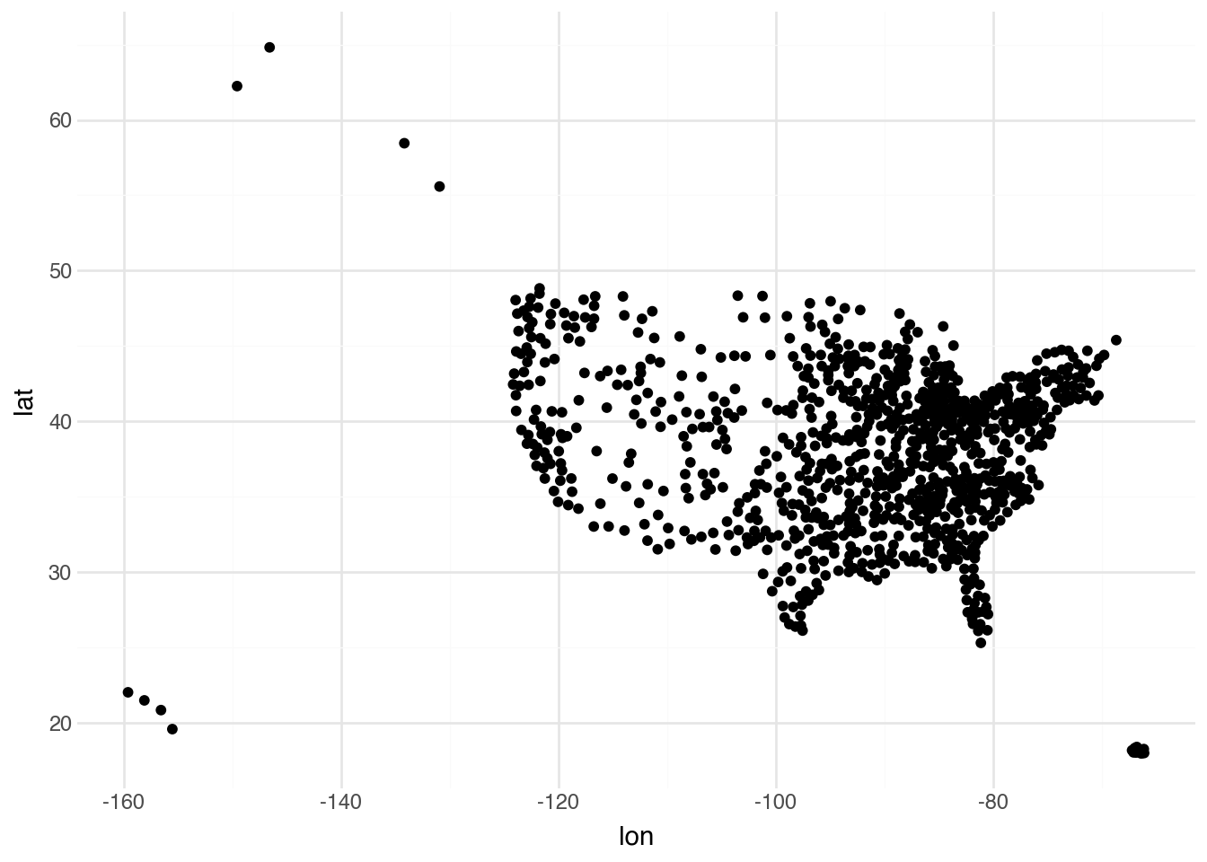
This scatter plot is functional but has several limitations. The most obvious is that it treats longitude and latitude as if they were ordinary Cartesian coordinates, when in fact they represent positions on a curved surface. The distortion is particularly noticeable at higher latitudes, where equal increments in longitude correspond to shorter physical distances. Additionally, we have no context for these points: no coastlines, state boundaries, or other geographic features to help orient the viewer.
To unlock more sophisticated spatial functionality, we need to convert our latitude and longitude columns into proper geometric objects. The DSGeo.from_latlon() method creates a new column called geometry that stores each point as a binary blob in a standardized format. This format encodes not just the coordinates but also metadata about the coordinate reference system.
metro = DSGeo.from_latlon(metro)
metro
shape: (934, 14)
| name | geoid | quad | lon | lat | pop | density | age_median | hh_income_median | percent_own | rent_1br_median | rent_perc_income | division | geometry |
|---|---|---|---|---|---|---|---|---|---|---|---|---|---|
| str | i64 | str | f64 | f64 | f64 | f64 | f64 | i64 | f64 | i64 | f64 | str | binary |
| "New York" | 35620 | "NE" | -74.101056 | 40.76877 | 20.011812 | 1051.306467 | 42.9 | 86445 | 55.3 | 1430 | 31.0 | "Middle Atlantic" | b"\x01\x01\x00\x00\x000\xadY\xb2w\x86R\xc0\x13\x04\xd7\x10gbD@" |
| "Los Angeles" | 31080 | "W" | -118.148722 | 34.219406 | 13.202558 | 1040.647281 | 41.6 | 81652 | 51.3 | 1468 | 33.6 | "Pacific" | b"\x01\x01\x00\x00\x00\x1d\xadx\xa7\x84\x89]\xc0[\xf9\x8c|\x15\x1cA@" |
| "Chicago" | 16980 | "NC" | -87.95882 | 41.700605 | 9.607711 | 508.629406 | 41.9 | 78790 | 68.9 | 1060 | 29.0 | "East North Central" | b"\x01\x01\x00\x00\x00\x07\x8boM]\xfdU\xc0F\xce\x0dn\xad\xd9D@" |
| "Dallas" | 19100 | "S" | -96.970508 | 32.84948 | 7.54334 | 323.181404 | 41.3 | 76916 | 64.1 | 1106 | 29.1 | "West South Central" | b"\x01\x01\x00\x00\x00\xaf\xe3\xc9\xcc\x1c>X\xc0\x82]\x16\xc0\xbbl@@" |
| "Houston" | 26420 | "S" | -95.401574 | 29.787083 | 7.048954 | 316.543514 | 41.0 | 72551 | 65.1 | 997 | 30.0 | "West South Central" | b"\x01\x01\x00\x00\x00gd\x01c\xb3\xd9W\xc0\x87\xbbJH~\xc9=@" |
| … | … | … | … | … | … | … | … | … | … | … | … | … | … |
| "Zapata" | 49820 | "S" | -99.168533 | 27.000573 | 0.013945 | 5.081383 | 41.4 | 34406 | 77.1 | 321 | 34.6 | "West South Central" | b"\x01\x01\x00\x00\x00$l\xfa=\xc9\xcaX\xc0\x15L[\x93%\x00;@" |
| "Ketchikan" | 28540 | "O" | -130.927217 | 55.582484 | 0.013939 | 1.046556 | 44.6 | 77820 | 67.5 | 946 | 31.2 | "Pacific" | b"\x01\x01\x00\x00\x00\x99\xe3\xda\xc3\xab]`\xc0\xc4\x90\x8f\xd8\x8e\xcaK@" |
| "Craig" | 18780 | "W" | -108.207523 | 40.618749 | 0.01324 | 1.077471 | 44.5 | 58583 | 72.8 | 485 | 29.0 | "Mountain" | b"\x01\x01\x00\x00\x00\x92\x88u\x0dH\x0d[\xc0\xe7Q\x16+3OD@" |
| "Vernon" | 46900 | "S" | -99.240853 | 34.080611 | 0.012887 | 5.086411 | 41.5 | 45262 | 62.0 | 503 | 22.0 | "West South Central" | b"\x01\x01\x00\x00\x00\xcf\x9a\x09!j\xcfX\xc0\xd3z\xccuQ\x0aA@" |
| "Lamesa" | 29500 | "S" | -101.947637 | 32.742488 | 0.012371 | 5.291467 | 41.1 | 42778 | 71.5 | 611 | 34.5 | "West South Central" | b"\x01\x01\x00\x00\x00oF\xe3\x15\xa6|Y\xc0R\xc7~\xdc\x09_@@" |
The DataFrame now contains a geometry column that appears as a series of binary values. While these values are not human-readable, they can be manipulated by specialized spatial functions that understand their internal structure.
16.4 Coordinate Systems (CRS)
One of the most important concepts in spatial data analysis is the coordinate reference system (CRS), sometimes called a spatial reference system. A CRS defines how coordinates map to actual locations on Earth. This might seem straightforward, but Earth’s surface is curved while maps are flat. Any attempt to represent the globe on a two-dimensional surface requires making trade-offs: you can preserve shapes or areas or distances, but never all three simultaneously.
The most common CRS for storing geographic data is WGS 84 (World Geodetic System 1984), which uses latitude and longitude measured in degrees. This is the system used by GPS devices and most web mapping services. When we created our geometry column above, the coordinates were assumed to be in WGS 84. However, for visualization and certain calculations, we often want to project our data into a different CRS that is optimized for a particular region or purpose.
Each CRS is identified by a numeric code in the EPSG (European Petroleum Survey Group) registry. For example:
- EPSG:4326 is WGS 84, the standard latitude/longitude system
- EPSG:5069 is NAD83 Conus Albers, an equal-area projection suitable for the contiguous United States
- EPSG:3857 is Web Mercator, used by Google Maps and other web mapping services
- EPSG:32618 is UTM Zone 18N, appropriate for the US East Coast
- EPSG:2154 is the official projection for Metropolitan France (including Corsica), mandated by French law
- EPSG:7791 is Italy’s modern national reference system and the most accurate for Italian data
To find the appropriate EPSG code for a specific region or purpose, you can search the EPSG.io website or consult the Spatial Reference database. These resources allow you to look up projections by name, region, or properties (such as whether they preserve area or shape).
When we plot our metro data with a specific CRS, the coordinates are transformed to reflect the chosen projection. The Albers Equal Area projection (EPSG:5069) is designed to minimize distortion for the contiguous United States, making it a good choice for visualizing data across the country.
DSGeo.plot(metro, crs=5069)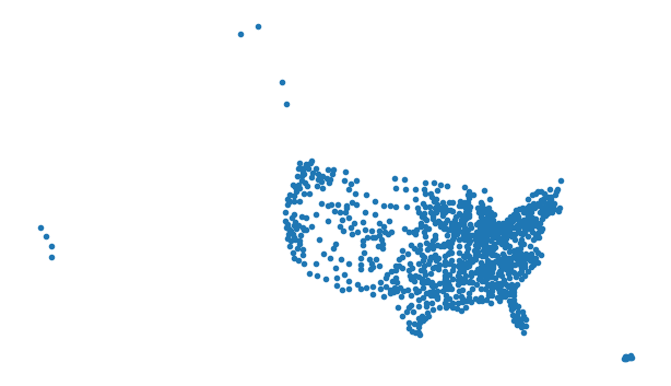
Notice how the shape of the point cloud now more closely resembles the familiar outline of the continental United States. Alaska and Hawaii, if present in the data, would appear distorted under this projection because it is optimized for the lower 48 states.
Why projections matter
The choice of projection can have significant implications for analysis. Consider calculating the distance between two cities. In WGS 84 coordinates, the distance between two points depends on their latitude: one degree of longitude represents about 111 kilometers at the equator but only about 85 kilometers at 40° latitude (roughly the latitude of New York). If you compute distances using raw latitude/longitude values as if they were Cartesian coordinates, your results will be systematically wrong.
Similarly, if you want to calculate the area of a state or country, you need to use an equal-area projection. Using a projection that distorts areas (like Web Mercator) will give you incorrect results. This is why Greenland appears larger than Africa on many web maps, even though Africa is actually 14 times larger.
16.5 Interactive Visualization
Static maps are useful for publications and reports, but interactive maps allow for exploration and discovery. The DSGeo.explore() function creates an interactive map powered by the Folium library, which in turn uses Leaflet.js. Users can zoom, pan, and click on features to see their attributes.
DSGeo.explore(metro, tooltip=[c.name])Make this Notebook Trusted to load map: File -> Trust Notebook
The tooltip parameter specifies which columns should be displayed when the user hovers over a point. Try zooming in on different regions and clicking on individual metro areas to see their names. The base map provides geographic context that was missing from our static scatter plot.
16.6 Spatial Polygons
While points are useful for representing discrete locations, many spatial phenomena are better represented as polygons: closed shapes that define the boundaries of regions. States, countries, zip codes, census tracts, and watersheds are all naturally represented as polygons. Each polygon is defined by a series of coordinate pairs that trace its boundary.
Spatial data is commonly stored in specialized file formats that can encode complex geometries along with their attributes. The GeoJSON format is particularly popular for web applications because it is based on JSON (JavaScript Object Notation) and can be read by virtually any programming language. GeoJSON files have a standardized structure where each row in the equivalent table is called a feature, and all features are collected into a FeatureCollection. The official specification is maintained by the Internet Engineering Task Force as RFC 7946.
Other common spatial formats include Shapefiles (a legacy format still widely used), GeoPackage (a modern SQLite-based format), and various database formats like PostGIS. Our DSGeo.read_file() function can read most of these formats.
state = DSGeo.read_file("data/acs_state.geojson")
state
shape: (50, 4)
| name | abb | fips | geometry |
|---|---|---|---|
| str | str | str | binary |
| "Maine" | "ME" | "23" | b"\x01\x06\x00\x00\x00\x01\x00\x00\x00\x01\x03\x00\x00\x00\x01\x00\x00\x00C\x00\x00\x00\x93\x15\xa7Z\x0b\xadQ\xc0\x10>yX\xa8\x87E@y\x15\x8cJ\xea\xb4Q\xc0\xb4\xe3\xa2ZD\x90E@\xda\xe2p\xe6W\xb4"… |
| "New Hampshire" | "NH" | "33" | b"\x01\x06\x00\x00\x00\x01\x00\x00\x00\x01\x03\x00\x00\x00\x01\x00\x00\x00!\x00\x00\x00\xeb\x1ag\xd3\x11\xe0Q\xc0a\xc2hV\xb6\x81F@4\x85\xb2\xf0\xf5\xd9Q\xc0#\x88f\x9e\\x99F@`\xc7G\x8b3\xd2"… |
| "Delaware" | "DE" | "10" | b"\x01\x06\x00\x00\x00\x01\x00\x00\x00\x01\x03\x00\x00\x00\x01\x00\x00\x00\x10\x00\x00\x00ip[[x\xf2R\xc0\x1a\x1aO\x04q\xdcC@\x1dr3\xdc\x80\xe7R\xc0X8I\xf3\xc7\xeaC@\xfe\xf34`\x90\xda"… |
| "South Carolina" | "SC" | "45" | b"\x01\x06\x00\x00\x00\x01\x00\x00\x00\x01\x03\x00\x00\x00\x01\x00\x00\x009\x00\x00\x00y\x89\x94f\xf3\xc6T\xc0\x8e\xb9\x17\x98\x15\x80A@\x9cI\xb7%r\x9dT\xc0s\x81\xcbc\xcd\x96A@\xda`S\xe7Q\x8b"… |
| "Nebraska" | "NE" | "31" | b"\x01\x06\x00\x00\x00\x01\x00\x00\x00\x01\x03\x00\x00\x00\x01\x00\x00\x00.\x00\x00\x00\x18\xe2\xc9nf\x03Z\xc0;\xefU+\x13\x80E@R\xf3U\xf2\xb1\xb2Y\xc0\xb9S:X\xff\x7fE@\xb7\x93\x16.\xabm"… |
| … | … | … | … |
| "Florida" | "FL" | "12" | b"\x01\x06\x00\x00\x00\x01\x00\x00\x00\x01\x03\x00\x00\x00\x01\x00\x00\x00t\x00\x00\x00Z\xd1\x90\xf1(@U\xc0%\xb2\x0f\xb2,\x00?@\x90rL\x16\xf7;U\xc0\x1du\xacRz\xe2>@)7\x19U\x86:"… |
| "Alaska" | "AK" | "02" | b"\x01\x06\x00\x00\x00\x01\x00\x00\x00\x01\x03\x00\x00\x00\x01\x00\x00\x00k\x02\x00\x009\xaf\xce1\x20\x04e\xc0\x16\xa3\xae\xb5\xf7iP@\xa1\x16-@[\xffd\xc0\xc7\x19\xdf\x17\x97nP@k\x90e\xc1D\xf1"… |
| "New Jersey" | "NJ" | "34" | b"\x01\x06\x00\x00\x00\x01\x00\x00\x00\x01\x03\x00\x00\x00\x01\x00\x00\x00$\x00\x00\x00T\xd9\xe8\x9c\x9f\xe0R\xc0M.\x00\x8d\xd2\xd7C@\xfe\xf34`\x90\xdaR\xc0-\x85#H\xa5\xe6C@\x8ft\xb1i\xa5\xc9"… |
| "North Dakota" | "ND" | "38" | b"\x01\x06\x00\x00\x00\x01\x00\x00\x00\x01\x03\x00\x00\x00\x01\x00\x00\x00\x19\x00\x00\x00X\xabw\xb8\x1d\x03Z\xc0\xab'\xd6\xa9\xf2\x7fH@\x00\xc9t\xe8\xf4\x8dY\xc01v\xa4\xfa\xce\x7fH@\xfe\x1e-\xce\x18H"… |
| "Iowa" | "IA" | "19" | b"\x01\x06\x00\x00\x00\x01\x00\x00\x00\x01\x03\x00\x00\x00\x01\x00\x00\x00<\x00\x00\x00O%;6\x02\x1dX\xc0\x7f\x9f\x8e\xc7\x0c\xc0E@F\xb5\xa5\x0e\xf2\xe0W\xc0]\xb5\x89\x93\xfb\xbfE@\xee\x10\x8d\xee\x20~"… |
The geometry column now contains polygon geometries rather than points. Each polygon is defined by many coordinate pairs (sometimes thousands for states with complex coastlines), but they are all stored efficiently in the binary geometry format.
Unlike point data, polygon data cannot be meaningfully visualized with a simple scatter plot. We need specialized functions that understand how to draw shapes from their vertex coordinates. The effect of projection is also much more noticeable with polygons than with points.
DSGeo.plot(state, crs=5069)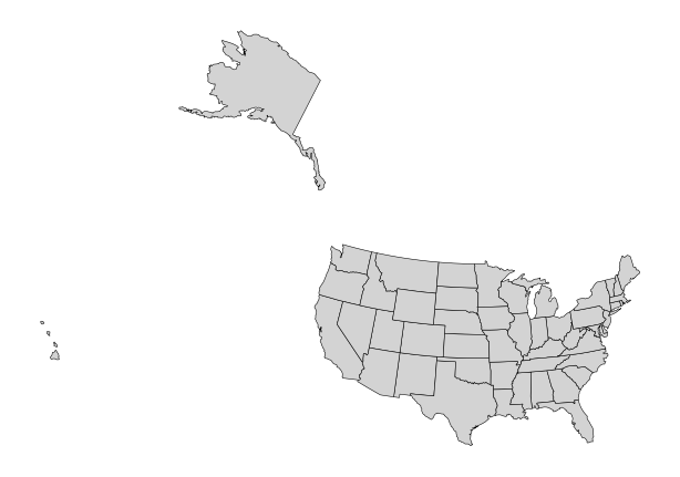
Compare this to what the same data would look like in unprojected coordinates. The familiar shapes of states would be distorted, particularly in the northern regions where lines of longitude converge. The Albers projection stretches and compresses the coordinates to create a more faithful representation of the true shapes and relative sizes of states.
Interactive maps work with polygons just as they do with points. Users can hover over states to see their names and other attributes.
DSGeo.explore(state, tooltip=[c.name])Make this Notebook Trusted to load map: File -> Trust Notebook
Other geometry types
Points and polygons are the most common geometry types, but GeoJSON and other spatial formats support several others:
- LineString: A sequence of connected points forming a path, useful for roads, rivers, or flight routes
- MultiPoint: A collection of points treated as a single feature
- MultiLineString: Multiple disconnected line segments treated as a single feature
- MultiPolygon: Multiple disconnected polygons treated as a single feature (useful for states with islands, like Hawaii)
- GeometryCollection: A heterogeneous collection containing any mix of the above types
Most of the techniques in this chapter apply to all geometry types, though some operations (like calculating area) only make sense for polygons.
16.7 Polygon Metrics
Once we have polygon geometries, we can compute various geometric properties. Two particularly useful properties are the centroid (the geometric center of a polygon) and the area (the amount of surface enclosed by the polygon’s boundary).
The centroid of a polygon is itself a point geometry. Adding centroids to our state data gives us a representative point location for each state, which can be useful for labeling maps or for spatial operations that require point geometries.
state = DSGeo.add_centroid(state)
state
shape: (50, 6)
| name | abb | fips | geometry | lon | lat |
|---|---|---|---|---|---|
| str | str | str | binary | f64 | f64 |
| "Maine" | "ME" | "23" | b"\x01\x06\x00\x00\x00\x01\x00\x00\x00\x01\x03\x00\x00\x00\x01\x00\x00\x00C\x00\x00\x00\x93\x15\xa7Z\x0b\xadQ\xc0\x10>yX\xa8\x87E@y\x15\x8cJ\xea\xb4Q\xc0\xb4\xe3\xa2ZD\x90E@\xda\xe2p\xe6W\xb4"… | -69.225019 | 45.368586 |
| "New Hampshire" | "NH" | "33" | b"\x01\x06\x00\x00\x00\x01\x00\x00\x00\x01\x03\x00\x00\x00\x01\x00\x00\x00!\x00\x00\x00\xeb\x1ag\xd3\x11\xe0Q\xc0a\xc2hV\xb6\x81F@4\x85\xb2\xf0\xf5\xd9Q\xc0#\x88f\x9e\\x99F@`\xc7G\x8b3\xd2"… | -71.579258 | 43.683295 |
| "Delaware" | "DE" | "10" | b"\x01\x06\x00\x00\x00\x01\x00\x00\x00\x01\x03\x00\x00\x00\x01\x00\x00\x00\x10\x00\x00\x00ip[[x\xf2R\xc0\x1a\x1aO\x04q\xdcC@\x1dr3\xdc\x80\xe7R\xc0X8I\xf3\xc7\xeaC@\xfe\xf34`\x90\xda"… | -75.501089 | 38.988027 |
| "South Carolina" | "SC" | "45" | b"\x01\x06\x00\x00\x00\x01\x00\x00\x00\x01\x03\x00\x00\x00\x01\x00\x00\x009\x00\x00\x00y\x89\x94f\xf3\xc6T\xc0\x8e\xb9\x17\x98\x15\x80A@\x9cI\xb7%r\x9dT\xc0s\x81\xcbc\xcd\x96A@\xda`S\xe7Q\x8b"… | -80.892889 | 33.904653 |
| "Nebraska" | "NE" | "31" | b"\x01\x06\x00\x00\x00\x01\x00\x00\x00\x01\x03\x00\x00\x00\x01\x00\x00\x00.\x00\x00\x00\x18\xe2\xc9nf\x03Z\xc0;\xefU+\x13\x80E@R\xf3U\xf2\xb1\xb2Y\xc0\xb9S:X\xff\x7fE@\xb7\x93\x16.\xabm"… | -99.810823 | 41.527493 |
| … | … | … | … | … | … |
| "Florida" | "FL" | "12" | b"\x01\x06\x00\x00\x00\x01\x00\x00\x00\x01\x03\x00\x00\x00\x01\x00\x00\x00t\x00\x00\x00Z\xd1\x90\xf1(@U\xc0%\xb2\x0f\xb2,\x00?@\x90rL\x16\xf7;U\xc0\x1du\xacRz\xe2>@)7\x19U\x86:"… | -82.50424 | 28.652783 |
| "Alaska" | "AK" | "02" | b"\x01\x06\x00\x00\x00\x01\x00\x00\x00\x01\x03\x00\x00\x00\x01\x00\x00\x00k\x02\x00\x009\xaf\xce1\x20\x04e\xc0\x16\xa3\xae\xb5\xf7iP@\xa1\x16-@[\xffd\xc0\xc7\x19\xdf\x17\x97nP@k\x90e\xc1D\xf1"… | -152.675093 | 64.489399 |
| "New Jersey" | "NJ" | "34" | b"\x01\x06\x00\x00\x00\x01\x00\x00\x00\x01\x03\x00\x00\x00\x01\x00\x00\x00$\x00\x00\x00T\xd9\xe8\x9c\x9f\xe0R\xc0M.\x00\x8d\xd2\xd7C@\xfe\xf34`\x90\xdaR\xc0-\x85#H\xa5\xe6C@\x8ft\xb1i\xa5\xc9"… | -74.660909 | 40.182638 |
| "North Dakota" | "ND" | "38" | b"\x01\x06\x00\x00\x00\x01\x00\x00\x00\x01\x03\x00\x00\x00\x01\x00\x00\x00\x19\x00\x00\x00X\xabw\xb8\x1d\x03Z\xc0\xab'\xd6\xa9\xf2\x7fH@\x00\xc9t\xe8\xf4\x8dY\xc01v\xa4\xfa\xce\x7fH@\xfe\x1e-\xce\x18H"… | -100.467458 | 47.446063 |
| "Iowa" | "IA" | "19" | b"\x01\x06\x00\x00\x00\x01\x00\x00\x00\x01\x03\x00\x00\x00\x01\x00\x00\x00<\x00\x00\x00O%;6\x02\x1dX\xc0\x7f\x9f\x8e\xc7\x0c\xc0E@F\xb5\xa5\x0e\xf2\xe0W\xc0]\xb5\x89\x93\xfb\xbfE@\xee\x10\x8d\xee\x20~"… | -93.500512 | 42.07356 |
The centroid column contains point geometries representing the center of each state. For roughly rectangular states like Colorado, the centroid falls near the geographic center. For states with irregular shapes or multiple disconnected parts, the centroid might fall outside the state’s actual boundary.
Calculating area requires a projection that preserves area relationships. If we compute areas in unprojected WGS 84 coordinates, the results would be meaningless numbers that do not correspond to actual square kilometers or square miles. By specifying a CRS, we ensure that the calculated areas reflect true surface measurements.
state = DSGeo.add_area(state, crs=5069)
state.sort(c.area).select(c.name, c.area)
shape: (50, 2)
| name | area |
|---|---|
| str | f64 |
| "Rhode Island" | 2765.092425 |
| "Delaware" | 5169.59288 |
| "Connecticut" | 12958.532624 |
| "Hawaii" | 15215.771452 |
| "New Jersey" | 20160.360977 |
| … | … |
| "New Mexico" | 314909.256017 |
| "Montana" | 380769.784499 |
| "California" | 409190.207104 |
| "Texas" | 687901.770044 |
| "Alaska" | 1.4557e6 |
The results show area in square meters (the default unit for most projected coordinate systems). Dividing by 1,000,000 would give square kilometers. As expected, Alaska is the largest state by far, followed by Texas and California.
16.8 Choropleth Maps
A choropleth map colors geographic regions according to the value of a variable. This type of visualization is extremely common for showing how quantities vary across space: election results by county, income levels by census tract, or disease rates by state. The column parameter tells the explore function which variable to use for coloring.
DSGeo.explore(state, column=c.area, tooltip=[c.name])Make this Notebook Trusted to load map: File -> Trust Notebook
The resulting map shows each state colored according to its area, with a legend indicating how colors correspond to values. Larger states appear darker (or whatever color scheme is in use), making spatial patterns immediately visible.
Choropleth maps are powerful but can be misleading. Because larger regions occupy more visual space, they can dominate the viewer’s attention even if they contain fewer people or are otherwise less important. For this reason, choropleth maps are best suited for variables that are naturally area-based (like population density) rather than absolute counts (like total population).
16.9 Spatial Joins
In Chapter 4, we learned how to join two tables based on a shared key column. Spatial joins extend this concept by joining tables based on their geometric relationships. Instead of matching rows where a key value is equal, we match rows where geometries intersect, touch, contain, or are within some distance of each other.
The most common spatial join matches points to the polygons that contain them. Given our metro areas (points) and states (polygons), we can determine which state contains each metro area by checking which state polygon each metro point falls inside.
DSGeo.sjoin(metro, state)
shape: (920, 21)
| name | geoid | quad | lon | lat | pop | density | age_median | hh_income_median | percent_own | rent_1br_median | rent_perc_income | division | index__right | name__right | abb | fips | lon__right | lat__right | area | geometry |
|---|---|---|---|---|---|---|---|---|---|---|---|---|---|---|---|---|---|---|---|---|
| str | i64 | str | f64 | f64 | f64 | f64 | f64 | i64 | f64 | i64 | f64 | str | i64 | str | str | str | f64 | f64 | f64 | binary |
| "New York" | 35620 | "NE" | -74.101056 | 40.76877 | 20.011812 | 1051.306467 | 42.9 | 86445 | 55.3 | 1430 | 31.0 | "Middle Atlantic" | 47 | "New Jersey" | "NJ" | "34" | -74.660909 | 40.182638 | 20160.360977 | b"\x01\x01\x00\x00\x000\xadY\xb2w\x86R\xc0\x13\x04\xd7\x10gbD@" |
| "Los Angeles" | 31080 | "W" | -118.148722 | 34.219406 | 13.202558 | 1040.647281 | 41.6 | 81652 | 51.3 | 1468 | 33.6 | "Pacific" | 9 | "California" | "CA" | "06" | -119.61258 | 37.252557 | 409190.207104 | b"\x01\x01\x00\x00\x00\x1d\xadx\xa7\x84\x89]\xc0[\xf9\x8c|\x15\x1cA@" |
| "Chicago" | 16980 | "NC" | -87.95882 | 41.700605 | 9.607711 | 508.629406 | 41.9 | 78790 | 68.9 | 1060 | 29.0 | "East North Central" | 28 | "Illinois" | "IL" | "17" | -89.196324 | 40.061609 | 145928.761225 | b"\x01\x01\x00\x00\x00\x07\x8boM]\xfdU\xc0F\xce\x0dn\xad\xd9D@" |
| "Dallas" | 19100 | "S" | -96.970508 | 32.84948 | 7.54334 | 323.181404 | 41.3 | 76916 | 64.1 | 1106 | 29.1 | "West South Central" | 8 | "Texas" | "TX" | "48" | -99.349969 | 31.484882 | 687901.770044 | b"\x01\x01\x00\x00\x00\xaf\xe3\xc9\xcc\x1c>X\xc0\x82]\x16\xc0\xbbl@@" |
| "Houston" | 26420 | "S" | -95.401574 | 29.787083 | 7.048954 | 316.543514 | 41.0 | 72551 | 65.1 | 997 | 30.0 | "West South Central" | 8 | "Texas" | "TX" | "48" | -99.349969 | 31.484882 | 687901.770044 | b"\x01\x01\x00\x00\x00gd\x01c\xb3\xd9W\xc0\x87\xbbJH~\xc9=@" |
| … | … | … | … | … | … | … | … | … | … | … | … | … | … | … | … | … | … | … | … | … |
| "Zapata" | 49820 | "S" | -99.168533 | 27.000573 | 0.013945 | 5.081383 | 41.4 | 34406 | 77.1 | 321 | 34.6 | "West South Central" | 8 | "Texas" | "TX" | "48" | -99.349969 | 31.484882 | 687901.770044 | b"\x01\x01\x00\x00\x00$l\xfa=\xc9\xcaX\xc0\x15L[\x93%\x00;@" |
| "Ketchikan" | 28540 | "O" | -130.927217 | 55.582484 | 0.013939 | 1.046556 | 44.6 | 77820 | 67.5 | 946 | 31.2 | "Pacific" | 46 | "Alaska" | "AK" | "02" | -152.675093 | 64.489399 | 1.4557e6 | b"\x01\x01\x00\x00\x00\x99\xe3\xda\xc3\xab]`\xc0\xc4\x90\x8f\xd8\x8e\xcaK@" |
| "Craig" | 18780 | "W" | -108.207523 | 40.618749 | 0.01324 | 1.077471 | 44.5 | 58583 | 72.8 | 485 | 29.0 | "Mountain" | 19 | "Colorado" | "CO" | "08" | -105.54769 | 38.997652 | 269556.293547 | b"\x01\x01\x00\x00\x00\x92\x88u\x0dH\x0d[\xc0\xe7Q\x16+3OD@" |
| "Vernon" | 46900 | "S" | -99.240853 | 34.080611 | 0.012887 | 5.086411 | 41.5 | 45262 | 62.0 | 503 | 22.0 | "West South Central" | 8 | "Texas" | "TX" | "48" | -99.349969 | 31.484882 | 687901.770044 | b"\x01\x01\x00\x00\x00\xcf\x9a\x09!j\xcfX\xc0\xd3z\xccuQ\x0aA@" |
| "Lamesa" | 29500 | "S" | -101.947637 | 32.742488 | 0.012371 | 5.291467 | 41.1 | 42778 | 71.5 | 611 | 34.5 | "West South Central" | 8 | "Texas" | "TX" | "48" | -99.349969 | 31.484882 | 687901.770044 | b"\x01\x01\x00\x00\x00oF\xe3\x15\xa6|Y\xc0R\xc7~\xdc\x09_@@" |
The result contains all columns from both DataFrames, with each metro area matched to the state it falls within. Metro areas that span state boundaries will be assigned to whichever state contains their center point (the coordinate we used when creating the point geometry). Notice that the geometry in the output is the point geometry from the first (left) DataFrame.
We can also reverse the order of the join to get state geometry in the result. When we put the states first, the output contains polygon geometries, with each state matched to the metro areas it contains.
DSGeo.sjoin(state, metro)
shape: (920, 21)
| name | abb | fips | lon | lat | area | index__right | name__right | geoid | quad | lon__right | lat__right | pop | density | age_median | hh_income_median | percent_own | rent_1br_median | rent_perc_income | division | geometry |
|---|---|---|---|---|---|---|---|---|---|---|---|---|---|---|---|---|---|---|---|---|
| str | str | str | f64 | f64 | f64 | i64 | str | i64 | str | f64 | f64 | f64 | f64 | f64 | i64 | f64 | i64 | f64 | str | binary |
| "Maine" | "ME" | "23" | -69.225019 | 45.368586 | 85262.523591 | 104 | "Portland" | 38860 | "NE" | -70.470321 | 43.695543 | 0.547792 | 93.194683 | 43.8 | 77759 | 76.8 | 968 | 28.9 | "New England" | b"\x01\x06\x00\x00\x00\x01\x00\x00\x00\x01\x03\x00\x00\x00\x01\x00\x00\x00C\x00\x00\x00\x93\x15\xa7Z\x0b\xadQ\xc0\x10>yX\xa8\x87E@y\x15\x8cJ\xea\xb4Q\xc0\xb4\xe3\xa2ZD\x90E@\xda\xe2p\xe6W\xb4"… |
| "Maine" | "ME" | "23" | -69.225019 | 45.368586 | 85262.523591 | 365 | "Lewiston" | 30340 | "NE" | -70.206499 | 44.16555 | 0.110378 | 85.911812 | 43.4 | 59287 | 70.1 | 674 | 28.0 | "New England" | b"\x01\x06\x00\x00\x00\x01\x00\x00\x00\x01\x03\x00\x00\x00\x01\x00\x00\x00C\x00\x00\x00\x93\x15\xa7Z\x0b\xadQ\xc0\x10>yX\xa8\x87E@y\x15\x8cJ\xea\xb4Q\xc0\xb4\xe3\xa2ZD\x90E@\xda\xe2p\xe6W\xb4"… |
| "Maine" | "ME" | "23" | -69.225019 | 45.368586 | 85262.523591 | 337 | "Augusta" | 12300 | "NE" | -69.767669 | 44.408937 | 0.123293 | 50.14378 | 44.9 | 58097 | 76.4 | 663 | 29.1 | "New England" | b"\x01\x06\x00\x00\x00\x01\x00\x00\x00\x01\x03\x00\x00\x00\x01\x00\x00\x00C\x00\x00\x00\x93\x15\xa7Z\x0b\xadQ\xc0\x10>yX\xa8\x87E@y\x15\x8cJ\xea\xb4Q\xc0\xb4\xe3\xa2ZD\x90E@\xda\xe2p\xe6W\xb4"… |
| "Maine" | "ME" | "23" | -69.225019 | 45.368586 | 85262.523591 | 287 | "Bangor" | 12620 | "NE" | -68.650949 | 45.397272 | 0.152211 | 16.55587 | 42.7 | 55125 | 73.8 | 720 | 29.0 | "New England" | b"\x01\x06\x00\x00\x00\x01\x00\x00\x00\x01\x03\x00\x00\x00\x01\x00\x00\x00C\x00\x00\x00\x93\x15\xa7Z\x0b\xadQ\xc0\x10>yX\xa8\x87E@y\x15\x8cJ\xea\xb4Q\xc0\xb4\xe3\xa2ZD\x90E@\xda\xe2p\xe6W\xb4"… |
| "New Hampshire" | "NH" | "33" | -71.579258 | 43.683295 | 24037.263031 | 130 | "Manchester" | 31700 | "NE" | -71.715762 | 42.915227 | 0.420504 | 182.271376 | 44.1 | 86930 | 70.8 | 1009 | 29.0 | "New England" | b"\x01\x06\x00\x00\x00\x01\x00\x00\x00\x01\x03\x00\x00\x00\x01\x00\x00\x00!\x00\x00\x00\xeb\x1ag\xd3\x11\xe0Q\xc0a\xc2hV\xb6\x81F@4\x85\xb2\xf0\xf5\xd9Q\xc0#\x88f\x9e\\x99F@`\xc7G\x8b3\xd2"… |
| … | … | … | … | … | … | … | … | … | … | … | … | … | … | … | … | … | … | … | … | … |
| "Iowa" | "IA" | "19" | -93.500512 | 42.07356 | 145800.681715 | 900 | "Storm Lake" | 44740 | "NC" | -95.151132 | 42.735419 | 0.020723 | 13.813099 | 41.9 | 53645 | 74.4 | 555 | 23.6 | "West North Central" | b"\x01\x06\x00\x00\x00\x01\x00\x00\x00\x01\x03\x00\x00\x00\x01\x00\x00\x00<\x00\x00\x00O%;6\x02\x1dX\xc0\x7f\x9f\x8e\xc7\x0c\xc0E@F\xb5\xa5\x0e\xf2\xe0W\xc0]\xb5\x89\x93\xfb\xbfE@\xee\x10\x8d\xee\x20~"… |
| "Iowa" | "IA" | "19" | -93.500512 | 42.07356 | 145800.681715 | 923 | "Spencer" | 43980 | "NC" | -95.150936 | 43.082492 | 0.01641 | 11.083706 | 46.4 | 52307 | 73.1 | 571 | 27.2 | "West North Central" | b"\x01\x06\x00\x00\x00\x01\x00\x00\x00\x01\x03\x00\x00\x00\x01\x00\x00\x00<\x00\x00\x00O%;6\x02\x1dX\xc0\x7f\x9f\x8e\xc7\x0c\xc0E@F\xb5\xa5\x0e\xf2\xe0W\xc0]\xb5\x89\x93\xfb\xbfE@\xee\x10\x8d\xee\x20~"… |
| "Iowa" | "IA" | "19" | -93.500512 | 42.07356 | 145800.681715 | 596 | "Mason City" | 32380 | "NC" | -93.26083 | 43.203198 | 0.050635 | 20.045526 | 43.9 | 58753 | 74.7 | 576 | 23.5 | "West North Central" | b"\x01\x06\x00\x00\x00\x01\x00\x00\x00\x01\x03\x00\x00\x00\x01\x00\x00\x00<\x00\x00\x00O%;6\x02\x1dX\xc0\x7f\x9f\x8e\xc7\x0c\xc0E@F\xb5\xa5\x0e\xf2\xe0W\xc0]\xb5\x89\x93\xfb\xbfE@\xee\x10\x8d\xee\x20~"… |
| "Iowa" | "IA" | "19" | -93.500512 | 42.07356 | 145800.681715 | 917 | "Spirit Lake" | 44020 | "NC" | -95.150806 | 43.377979 | 0.017536 | 16.791337 | 44.6 | 65215 | 83.1 | 770 | 30.0 | "West North Central" | b"\x01\x06\x00\x00\x00\x01\x00\x00\x00\x01\x03\x00\x00\x00\x01\x00\x00\x00<\x00\x00\x00O%;6\x02\x1dX\xc0\x7f\x9f\x8e\xc7\x0c\xc0E@F\xb5\xa5\x0e\xf2\xe0W\xc0]\xb5\x89\x93\xfb\xbfE@\xee\x10\x8d\xee\x20~"… |
| "Iowa" | "IA" | "19" | -93.500512 | 42.07356 | 145800.681715 | 260 | "Waterloo" | 47940 | "NC" | -92.471855 | 42.536019 | 0.168595 | 43.066768 | 39.2 | 61632 | 71.2 | 625 | 27.9 | "West North Central" | b"\x01\x06\x00\x00\x00\x01\x00\x00\x00\x01\x03\x00\x00\x00\x01\x00\x00\x00<\x00\x00\x00O%;6\x02\x1dX\xc0\x7f\x9f\x8e\xc7\x0c\xc0E@F\xb5\xa5\x0e\xf2\xe0W\xc0]\xb5\x89\x93\xfb\xbfE@\xee\x10\x8d\xee\x20~"… |
This produces more rows than we have states because each state can contain multiple metro areas. The logic is analogous to a one-to-many relational join: the state geometry is duplicated for each metro area it contains.
Spatial joins can use various predicates (spatial relationships) beyond simple containment. The predicate parameter specifies which relationship to test. For example, we can find which states share a border with which other states using the touches predicate.
DSGeo.sjoin(state, state, predicate="touches")
shape: (214, 14)
| name | abb | fips | lon | lat | area | index__right | name__right | abb__right | fips__right | lon__right | lat__right | area__right | geometry |
|---|---|---|---|---|---|---|---|---|---|---|---|---|---|
| str | str | str | f64 | f64 | f64 | i64 | str | str | str | f64 | f64 | f64 | binary |
| "Maine" | "ME" | "23" | -69.225019 | 45.368586 | 85262.523591 | 1 | "New Hampshire" | "NH" | "33" | -71.579258 | 43.683295 | 24037.263031 | b"\x01\x06\x00\x00\x00\x01\x00\x00\x00\x01\x03\x00\x00\x00\x01\x00\x00\x00C\x00\x00\x00\x93\x15\xa7Z\x0b\xadQ\xc0\x10>yX\xa8\x87E@y\x15\x8cJ\xea\xb4Q\xc0\xb4\xe3\xa2ZD\x90E@\xda\xe2p\xe6W\xb4"… |
| "New Hampshire" | "NH" | "33" | -71.579258 | 43.683295 | 24037.263031 | 43 | "Massachusetts" | "MA" | "25" | -71.844911 | 42.278432 | 20631.817699 | b"\x01\x06\x00\x00\x00\x01\x00\x00\x00\x01\x03\x00\x00\x00\x01\x00\x00\x00!\x00\x00\x00\xeb\x1ag\xd3\x11\xe0Q\xc0a\xc2hV\xb6\x81F@4\x85\xb2\xf0\xf5\xd9Q\xc0#\x88f\x9e\\x99F@`\xc7G\x8b3\xd2"… |
| "New Hampshire" | "NH" | "33" | -71.579258 | 43.683295 | 24037.263031 | 29 | "Vermont" | "VT" | "50" | -72.66144 | 44.078034 | 24839.475007 | b"\x01\x06\x00\x00\x00\x01\x00\x00\x00\x01\x03\x00\x00\x00\x01\x00\x00\x00!\x00\x00\x00\xeb\x1ag\xd3\x11\xe0Q\xc0a\xc2hV\xb6\x81F@4\x85\xb2\xf0\xf5\xd9Q\xc0#\x88f\x9e\\x99F@`\xc7G\x8b3\xd2"… |
| "New Hampshire" | "NH" | "33" | -71.579258 | 43.683295 | 24037.263031 | 0 | "Maine" | "ME" | "23" | -69.225019 | 45.368586 | 85262.523591 | b"\x01\x06\x00\x00\x00\x01\x00\x00\x00\x01\x03\x00\x00\x00\x01\x00\x00\x00!\x00\x00\x00\xeb\x1ag\xd3\x11\xe0Q\xc0a\xc2hV\xb6\x81F@4\x85\xb2\xf0\xf5\xd9Q\xc0#\x88f\x9e\\x99F@`\xc7G\x8b3\xd2"… |
| "Delaware" | "DE" | "10" | -75.501089 | 38.988027 | 5169.59288 | 33 | "Maryland" | "MD" | "24" | -76.773391 | 39.040321 | 26772.630334 | b"\x01\x06\x00\x00\x00\x01\x00\x00\x00\x01\x03\x00\x00\x00\x01\x00\x00\x00\x10\x00\x00\x00ip[[x\xf2R\xc0\x1a\x1aO\x04q\xdcC@\x1dr3\xdc\x80\xe7R\xc0X8I\xf3\xc7\xeaC@\xfe\xf34`\x90\xda"… |
| … | … | … | … | … | … | … | … | … | … | … | … | … | … |
| "Iowa" | "IA" | "19" | -93.500512 | 42.07356 | 145800.681715 | 37 | "Missouri" | "MO" | "29" | -92.477487 | 38.367533 | 180621.339618 | b"\x01\x06\x00\x00\x00\x01\x00\x00\x00\x01\x03\x00\x00\x00\x01\x00\x00\x00<\x00\x00\x00O%;6\x02\x1dX\xc0\x7f\x9f\x8e\xc7\x0c\xc0E@F\xb5\xa5\x0e\xf2\xe0W\xc0]\xb5\x89\x93\xfb\xbfE@\xee\x10\x8d\xee\x20~"… |
| "Iowa" | "IA" | "19" | -93.500512 | 42.07356 | 145800.681715 | 28 | "Illinois" | "IL" | "17" | -89.196324 | 40.061609 | 145928.761225 | b"\x01\x06\x00\x00\x00\x01\x00\x00\x00\x01\x03\x00\x00\x00\x01\x00\x00\x00<\x00\x00\x00O%;6\x02\x1dX\xc0\x7f\x9f\x8e\xc7\x0c\xc0E@F\xb5\xa5\x0e\xf2\xe0W\xc0]\xb5\x89\x93\xfb\xbfE@\xee\x10\x8d\xee\x20~"… |
| "Iowa" | "IA" | "19" | -93.500512 | 42.07356 | 145800.681715 | 14 | "Wisconsin" | "WI" | "55" | -90.012344 | 44.630868 | 145016.280762 | b"\x01\x06\x00\x00\x00\x01\x00\x00\x00\x01\x03\x00\x00\x00\x01\x00\x00\x00<\x00\x00\x00O%;6\x02\x1dX\xc0\x7f\x9f\x8e\xc7\x0c\xc0E@F\xb5\xa5\x0e\xf2\xe0W\xc0]\xb5\x89\x93\xfb\xbfE@\xee\x10\x8d\xee\x20~"… |
| "Iowa" | "IA" | "19" | -93.500512 | 42.07356 | 145800.681715 | 32 | "Minnesota" | "MN" | "27" | -94.309123 | 46.315559 | 218497.340682 | b"\x01\x06\x00\x00\x00\x01\x00\x00\x00\x01\x03\x00\x00\x00\x01\x00\x00\x00<\x00\x00\x00O%;6\x02\x1dX\xc0\x7f\x9f\x8e\xc7\x0c\xc0E@F\xb5\xa5\x0e\xf2\xe0W\xc0]\xb5\x89\x93\xfb\xbfE@\xee\x10\x8d\xee\x20~"… |
| "Iowa" | "IA" | "19" | -93.500512 | 42.07356 | 145800.681715 | 7 | "South Dakota" | "SD" | "46" | -100.232438 | 44.436377 | 199692.46709 | b"\x01\x06\x00\x00\x00\x01\x00\x00\x00\x01\x03\x00\x00\x00\x01\x00\x00\x00<\x00\x00\x00O%;6\x02\x1dX\xc0\x7f\x9f\x8e\xc7\x0c\xc0E@F\xb5\xa5\x0e\xf2\xe0W\xc0]\xb5\x89\x93\xfb\xbfE@\xee\x10\x8d\xee\x20~"… |
This self-join matches each state to every other state that shares at least one point on its boundary. The result shows all pairs of neighboring states. Notice that each border appears twice: California touches Oregon, and Oregon touches California. If you only want each pair once, you would need to filter or deduplicate the results.
Other useful predicates include:
- intersects: Geometries share any space (including boundaries)
- contains: The first geometry completely encloses the second
- within: The first geometry is completely enclosed by the second
- crosses: Geometries share some but not all interior points
- overlaps: Geometries share some space but neither contains the other
16.10 Nearest Neighbor Joins
Sometimes we want to match features not based on overlap or containment but based on proximity. The sjoin_nearest function finds, for each feature in the first DataFrame, the closest feature in the second DataFrame. This is useful for questions like “What is the nearest hospital to each school?” or “Which weather station is closest to each measurement location?”
DSGeo.sjoin_nearest(metro, metro, exclusive=True)
shape: (934, 28)
| name | geoid | quad | lon | lat | pop | density | age_median | hh_income_median | percent_own | rent_1br_median | rent_perc_income | division | index_right | name_right | geoid_right | quad_right | lon_right | lat_right | pop_right | density_right | age_median_right | hh_income_median_right | percent_own_right | rent_1br_median_right | rent_perc_income_right | division_right | geometry |
|---|---|---|---|---|---|---|---|---|---|---|---|---|---|---|---|---|---|---|---|---|---|---|---|---|---|---|---|
| str | i64 | str | f64 | f64 | f64 | f64 | f64 | i64 | f64 | i64 | f64 | str | i64 | str | i64 | str | f64 | f64 | f64 | f64 | f64 | i64 | f64 | i64 | f64 | str | binary |
| "New York" | 35620 | "NE" | -74.101056 | 40.76877 | 20.011812 | 1051.306467 | 42.9 | 86445 | 55.3 | 1430 | 31.0 | "Middle Atlantic" | 141 | "Trenton" | 45940 | "NE" | -74.701703 | 40.283417 | 0.384951 | 650.172055 | 44.7 | 85687 | 65.7 | 1126 | 30.2 | "Middle Atlantic" | b"\x01\x01\x00\x00\x000\xadY\xb2w\x86R\xc0\x13\x04\xd7\x10gbD@" |
| "Los Angeles" | 31080 | "W" | -118.148722 | 34.219406 | 13.202558 | 1040.647281 | 41.6 | 81652 | 51.3 | 1468 | 33.6 | "Pacific" | 70 | "Oxnard" | 37100 | "W" | -119.083405 | 34.45556 | 0.845255 | 175.81324 | 42.1 | 94150 | 63.3 | 1582 | 34.2 | "Pacific" | b"\x01\x01\x00\x00\x00\x1d\xadx\xa7\x84\x89]\xc0[\xf9\x8c|\x15\x1cA@" |
| "Chicago" | 16980 | "NC" | -87.95882 | 41.700605 | 9.607711 | 508.629406 | 41.9 | 78790 | 68.9 | 1060 | 29.0 | "East North Central" | 368 | "Kankakee" | 28100 | "NC" | -87.861944 | 41.137788 | 0.108104 | 61.34992 | 41.8 | 61664 | 70.4 | 701 | 30.5 | "East North Central" | b"\x01\x01\x00\x00\x00\x07\x8boM]\xfdU\xc0F\xce\x0dn\xad\xd9D@" |
| "Dallas" | 19100 | "S" | -96.970508 | 32.84948 | 7.54334 | 323.181404 | 41.3 | 76916 | 64.1 | 1106 | 29.1 | "West South Central" | 685 | "Gainesville" | 23620 | "S" | -97.212584 | 33.639178 | 0.041215 | 17.700303 | 42.5 | 63338 | 69.6 | 666 | 25.0 | "West South Central" | b"\x01\x01\x00\x00\x00\xaf\xe3\xc9\xcc\x1c>X\xc0\x82]\x16\xc0\xbbl@@" |
| "Houston" | 26420 | "S" | -95.401574 | 29.787083 | 7.048954 | 316.543514 | 41.0 | 72551 | 65.1 | 997 | 30.0 | "West South Central" | 683 | "El Campo" | 20900 | "S" | -96.222207 | 29.277782 | 0.041602 | 14.65937 | 41.8 | 53963 | 69.2 | 600 | 26.3 | "West South Central" | b"\x01\x01\x00\x00\x00gd\x01c\xb3\xd9W\xc0\x87\xbbJH~\xc9=@" |
| … | … | … | … | … | … | … | … | … | … | … | … | … | … | … | … | … | … | … | … | … | … | … | … | … | … | … | … |
| "Zapata" | 49820 | "S" | -99.168533 | 27.000573 | 0.013945 | 5.081383 | 41.4 | 34406 | 77.1 | 321 | 34.6 | "West South Central" | 501 | "Rio Grande City" | 40100 | "S" | -98.738748 | 26.562072 | 0.065568 | 20.57443 | 40.5 | 33334 | 75.3 | 390 | 32.5 | "West South Central" | b"\x01\x01\x00\x00\x00$l\xfa=\xc9\xcaX\xc0\x15L[\x93%\x00;@" |
| "Ketchikan" | 28540 | "O" | -130.927217 | 55.582484 | 0.013939 | 1.046556 | 44.6 | 77820 | 67.5 | 946 | 31.2 | "Pacific" | 799 | "Juneau" | 27940 | "O" | -134.169542 | 58.45342 | 0.03224 | 4.445802 | 41.8 | 90126 | 68.5 | 1095 | 25.0 | "Pacific" | b"\x01\x01\x00\x00\x00\x99\xe3\xda\xc3\xab]`\xc0\xc4\x90\x8f\xd8\x8e\xcaK@" |
| "Craig" | 18780 | "W" | -108.207523 | 40.618749 | 0.01324 | 1.077471 | 44.5 | 58583 | 72.8 | 485 | 29.0 | "Mountain" | 864 | "Steamboat Springs" | 44460 | "W" | -106.990829 | 40.484142 | 0.024899 | 4.063905 | 41.4 | 83725 | 76.2 | 1371 | 29.7 | "Mountain" | b"\x01\x01\x00\x00\x00\x92\x88u\x0dH\x0d[\xc0\xe7Q\x16+3OD@" |
| "Vernon" | 46900 | "S" | -99.240853 | 34.080611 | 0.012887 | 5.086411 | 41.5 | 45262 | 62.0 | 503 | 22.0 | "West South Central" | 861 | "Altus" | 11060 | "S" | -99.414999 | 34.587933 | 0.02496 | 11.981281 | 40.8 | 55551 | 62.7 | 489 | 23.4 | "West South Central" | b"\x01\x01\x00\x00\x00\xcf\x9a\x09!j\xcfX\xc0\xd3z\xccuQ\x0aA@" |
| "Lamesa" | 29500 | "S" | -101.947637 | 32.742488 | 0.012371 | 5.291467 | 41.1 | 42778 | 71.5 | 611 | 34.5 | "West South Central" | 253 | "Midland" | 33260 | "S" | -101.991236 | 32.08914 | 0.172177 | 36.548597 | 38.9 | 87812 | 70.7 | 1128 | 26.8 | "West South Central" | b"\x01\x01\x00\x00\x00oF\xe3\x15\xa6|Y\xc0R\xc7~\xdc\x09_@@" |
Here we join the metro dataset to itself to find each metro area’s nearest neighbor. The exclusive=True parameter prevents each metro area from matching with itself (which would always be distance zero). The result shows pairs of metro areas that are nearest neighbors, along with the distance between them.
Nearest neighbor joins are computationally expensive because they potentially require comparing every feature in the first DataFrame to every feature in the second. For large datasets, this can be slow. Spatial libraries use sophisticated indexing structures (like R-trees) to speed up these queries, but they still scale less favorably than simple predicate-based joins.
16.11 Best Practices
Working with spatial data introduces several potential sources of error that do not arise with ordinary tabular data.
CRS mismatches: If two datasets use different coordinate reference systems, spatial operations will give incorrect results. Points might appear to be in the wrong location, or spatial joins might fail to find matches. Always verify that your datasets are in compatible CRSs before performing spatial operations, and transform them to a common CRS if necessary.
Unprojected coordinates for calculations: Never calculate distances or areas using raw latitude/longitude coordinates as if they were Cartesian. The errors can be substantial, especially for features that span large areas or are located far from the equator. Always project your data to an appropriate CRS first.
Polygon validity: Complex polygons can sometimes become geometrically invalid due to self-intersections or other topological errors. Many spatial functions will fail or give incorrect results on invalid geometries. If you encounter strange errors, check whether your geometries are valid and repair them if necessary.
Boundary effects: Features that span boundaries between regions can cause problems for spatial joins. A metro area that straddles a state line might be assigned to one state or the other depending on where its center point falls. Be aware of these edge cases and handle them appropriately for your analysis.