import numpy as np
import polars as pl

from funs import *
from plotnine import *
from polars import col as c
theme_set(theme_minimal())

import torch
import torch.nn as nn
import torch.optim as optim
from gensim.models import Word2Vec

mnist = pl.read_csv("data/mnist_1000.csv")
imdb5k = pl.read_parquet("data/imdb5k_pca.parquet")14 CNNs and Word2Vec
14.1 Setup
Load all of the modules and datasets needed for the chapter. We also load several parts of the torch module for building deep learning models and the Word2Vec model from gensim.
14.2 CNNs: Theory
The dense neural network we built in Chapter 13 treats each pixel as an independent feature. While this works reasonably well for small images like MNIST digits, it ignores a fundamental property of images: spatial structure. Pixels that are close together tend to be related. An edge in an image is defined by the relationship between neighboring pixels, not by any single pixel in isolation. Convolutional neural networks (CNNs) are designed to exploit this spatial structure by using a different type of layer that processes local regions of the input.
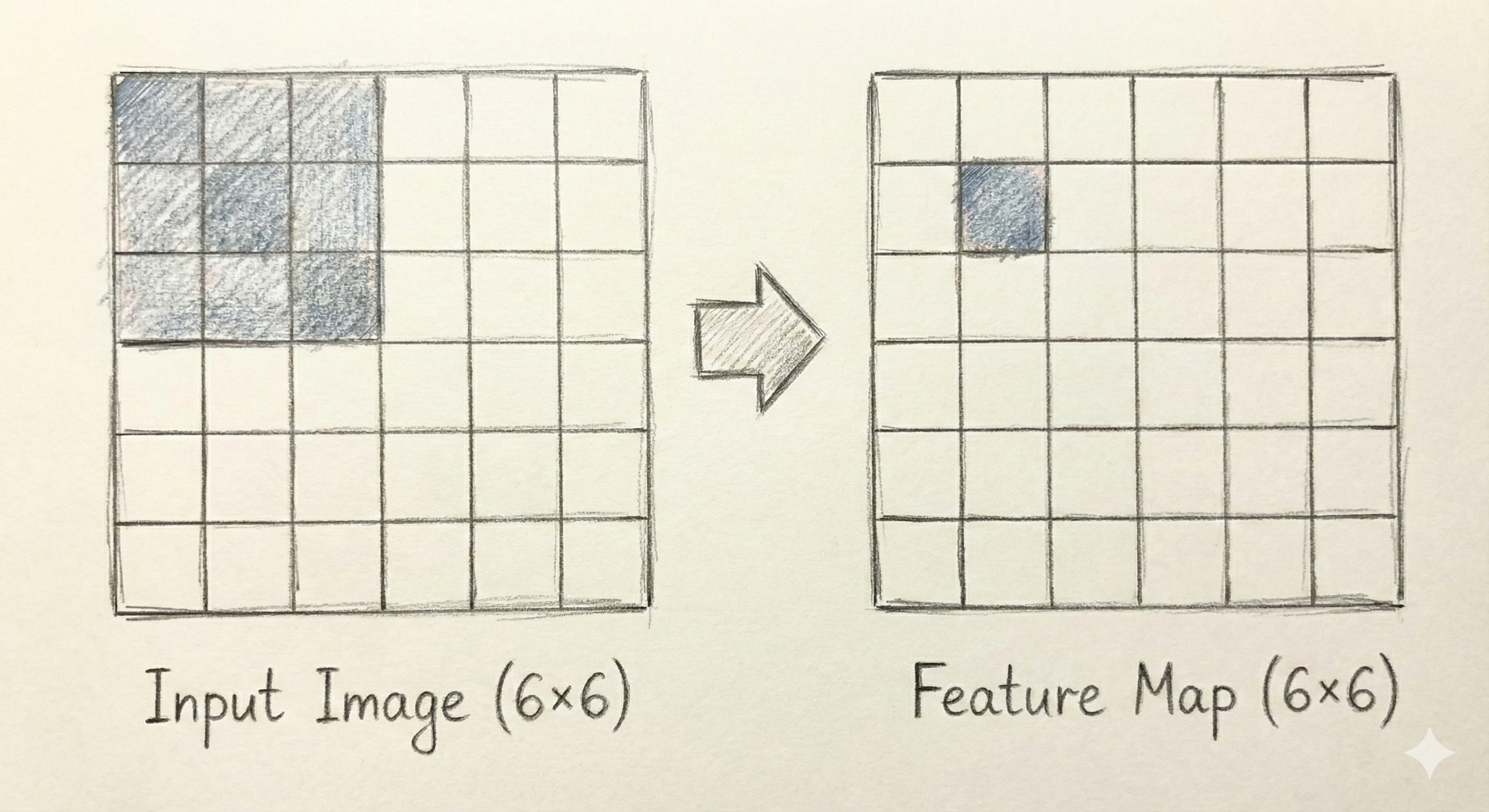
The core building block of a CNN is the convolutional layer. Instead of connecting every input to every output as in a dense layer, a convolutional layer applies a small filter (also called a kernel) that slides across the image. The filter is a small grid of weights, typically 3×3 or 5×5 pixels. At each position, the filter computes a weighted sum of the pixels it covers, producing a single output value. Figure Figure 14.1 illustrates this process for a 3×3 kernel applied to a small portion of an image.
The power of convolution comes from weight sharing: the same filter weights are used at every position in the image. This dramatically reduces the number of parameters compared to a dense layer. A 3×3 filter has only 9 weights (plus a bias term), regardless of the image size. Moreover, because the same filter is applied everywhere, it can detect the same pattern wherever it appears in the image. A filter that detects vertical edges will find them whether they appear in the top-left corner or the bottom-right.
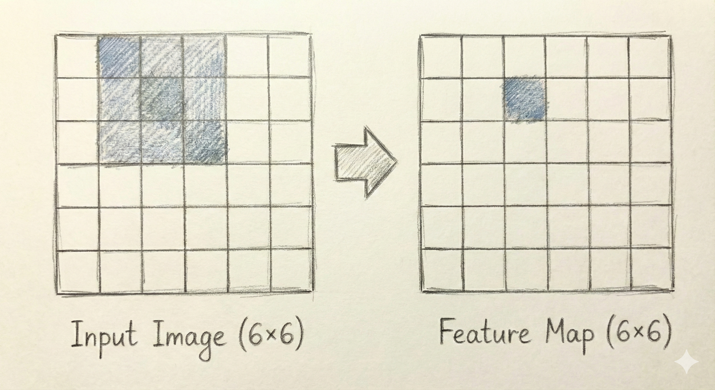
By sliding the filter across the entire image, we produce an output that has the same spatial structure as the input but with different values at each position. Figure Figure 14.2 illustrates how the kernel would get applied to another set of pixels in the image.
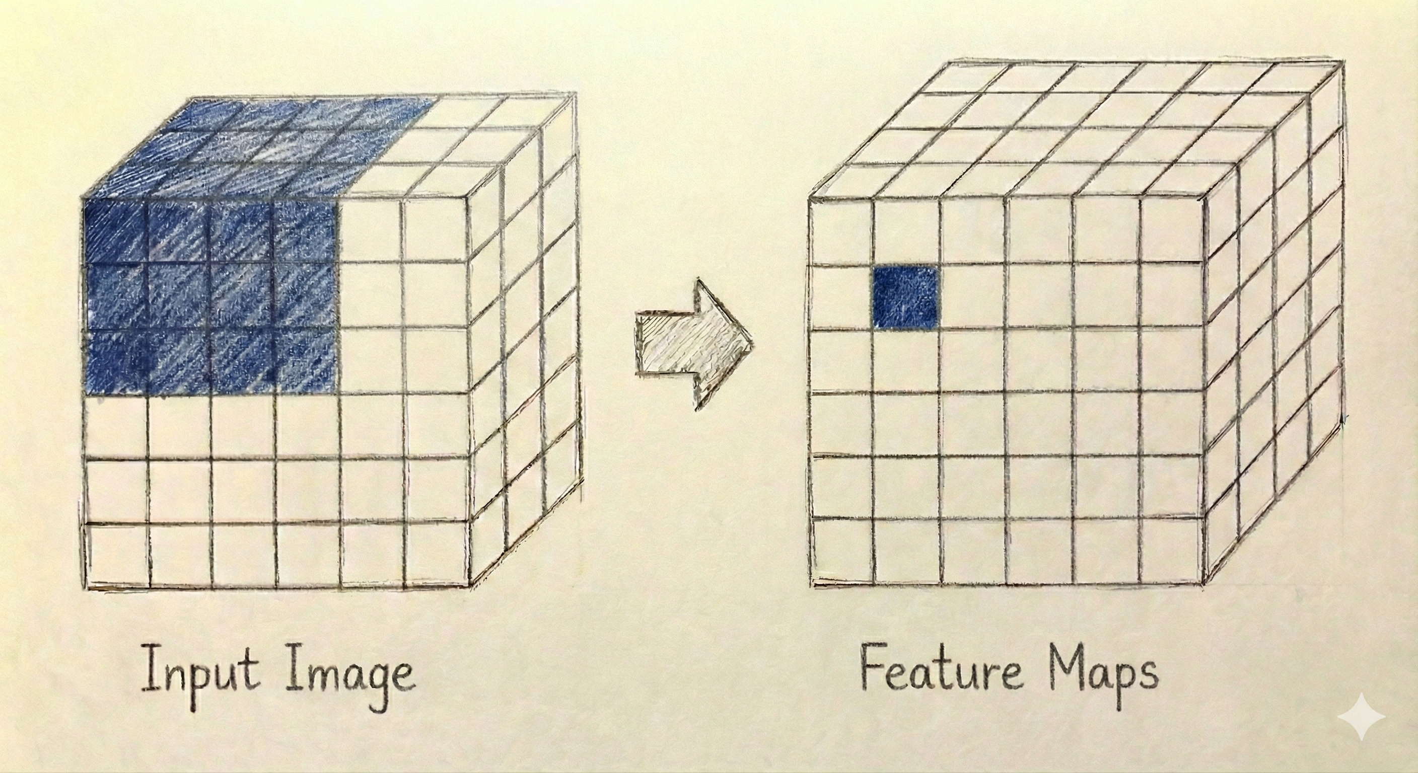
So far we have considered an input image that has only a height and a width and a single kernel. We can expand both the input and the output in a third dimension.
When working with color images, though, we have a third dimension corresponding to the red, green, and blue color channels. When we have a kernel, it will use all channels from the pixels in question. So, a 3×3 kernel for a color image would need \(3×3×3+1=28\) parameters. In practice, a convolutional layer also applies multiple filters simultaneously, each producing its own output. These outputs are stacked together to form a multi-channel result. If we apply 16 different filters to an image, we get 16 different feature maps, each highlighting different patterns in the input. A second convolution could be applied afterwards the works the same way, combining all of the filters within a spatial region. Figure Figure 14.3 illustrates how multiple filters produce multiple output channels from a color image.
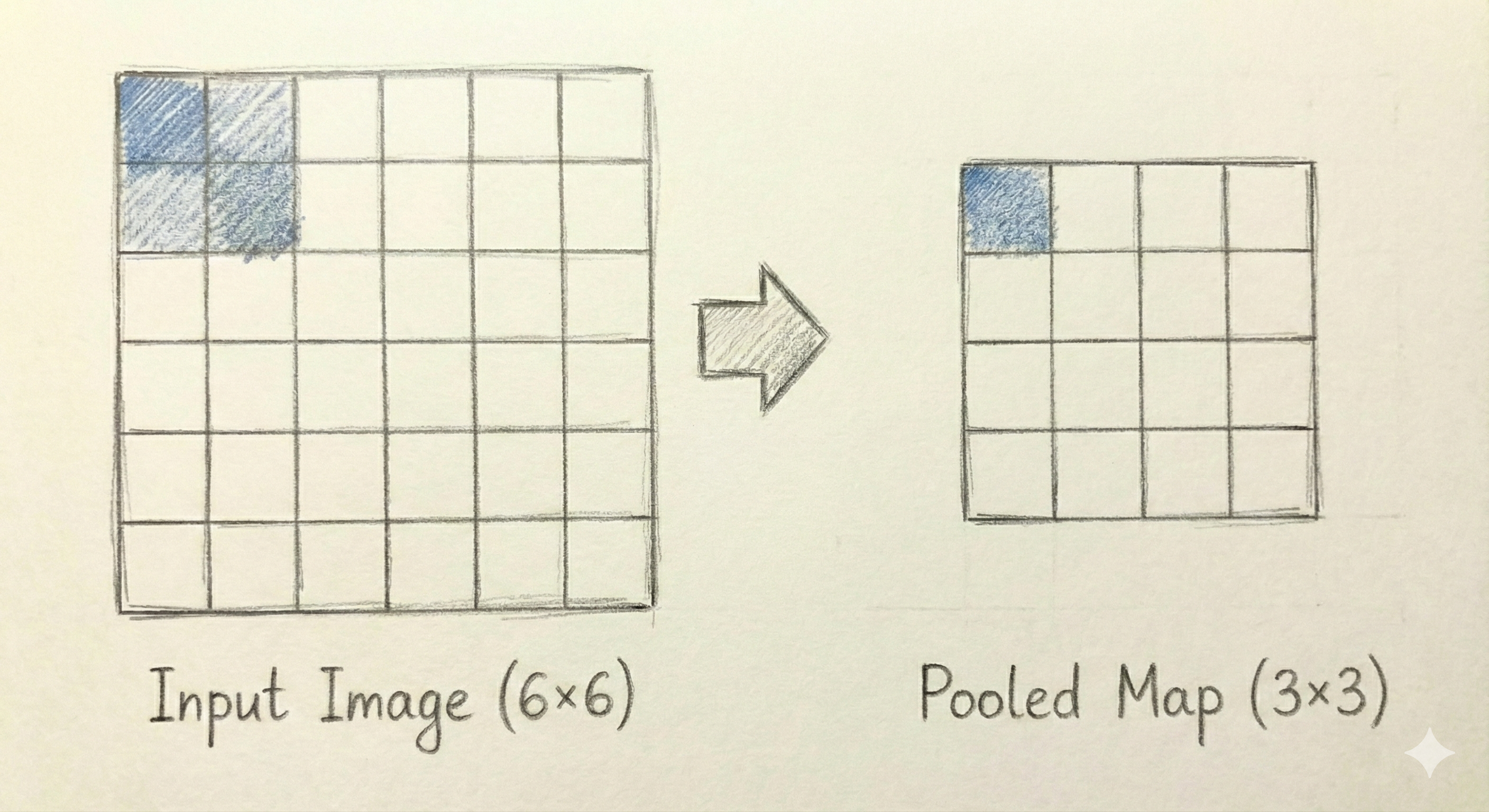
A second key component of CNNs is the pooling layer, which reduces the spatial dimensions of the feature maps. The most common type is max pooling, which divides the input into non-overlapping rectangular regions and outputs the maximum value from each region. A 2×2 max pooling operation reduces each dimension by half, so a 28×28 feature map becomes 14×14. Pooling serves two purposes: it reduces the computational burden for subsequent layers, and it provides a degree of translation invariance, meaning that small shifts in the input do not dramatically change the output. Figure Figure 14.4 shows how max pooling works on a small example.
A typical CNN architecture alternates between convolutional layers (followed by ReLU activations) and pooling layers. The convolutional layers detect increasingly complex features: early layers might detect edges and simple textures, while deeper layers combine these into more abstract representations like shapes or object parts. The pooling layers progressively reduce the spatial dimensions. After several such blocks, the feature maps are flattened into a vector and passed through one or more dense layers, which produce the final classification output. This combination of local feature detection through convolution and global reasoning through dense layers has proven remarkably effective across a wide range of image analysis tasks.
14.3 CNNs: Application
To apply a CNN to our MNIST data, we first need to reload the image data without flattening. Convolutional layers expect inputs with spatial structure: height, width, and channels. For our grayscale digits, each image is 28 pixels tall, 28 pixels wide, and has 1 channel.
X, X_train, X_test, y, y_train, y_test, cn = DSTorch.load_image(
    mnist, scale=True
)
X.shape
torch.Size([1000, 1, 28, 28])The shape shows that we have 1,000 images, each with 1 channel and dimensions 28×28. This four-dimensional structure (batch size, channels, height, width) is the standard format for image data in PyTorch.
We now define a CNN architecture using the same class-based approach as before. The model consists of two main parts: a feature extraction section with convolutional and pooling layers, and a classification section with dense layers.
class SimpleCNN(nn.Module):
    def __init__(self, num_classes=10):
        super().__init__()

        self.net = nn.Sequential(
            nn.Conv2d(1, 16, kernel_size=3, padding=1),
            nn.ReLU(),
            nn.MaxPool2d(2),

            nn.Conv2d(16, 32, kernel_size=3, padding=1),
            nn.ReLU(),
            nn.MaxPool2d(2),

            nn.Flatten(),
            nn.Linear(32 * 7 * 7, 128),
            nn.ReLU(),
            nn.Linear(128, num_classes)
        )

    def forward(self, x):
        return self.net(x)
The feature extraction section begins with nn.Conv2d(1, 16, kernel_size=3, padding=1). This creates a convolutional layer that takes 1 input channel (grayscale) and produces 16 output channels using 3×3 filters. The padding=1 argument adds a border of zeros around the input so that the output has the same spatial dimensions as the input. After the ReLU activation, nn.MaxPool2d(2) applies 2×2 max pooling, which halves both spatial dimensions from 28×28 to 14×14. The second convolutional block follows the same pattern: a 3×3 convolution that increases from 16 to 32 channels, a ReLU activation, and another 2×2 max pooling that reduces dimensions to 7×7. After these two blocks, each image is represented by a 32×7×7 tensor containing 1,568 values.
The classifier section first flattens this tensor into a vector of length \(32 \times 7 \times 7 = 1{,}568\). A dense layer reduces this to 128 hidden units, followed by ReLU and a final layer that produces 10 outputs for our 10 digit classes.
We create the model and optimizer, using a smaller learning rate than we did for the dense network. CNNs often benefit from lower learning rates because the shared weights across spatial positions can lead to larger effective gradients.
model = SimpleCNN()
optimizer = optim.Adam(model.parameters(), lr=1e-3)

DSTorch.train(
    model, optimizer, X_train, y_train, num_epochs=20, batch_size=64
)
Epoch 1/20, Loss: 2.4326
Epoch 2/20, Loss: 1.9463
Epoch 3/20, Loss: 1.1570
Epoch 4/20, Loss: 0.6653
Epoch 5/20, Loss: 0.4725
Epoch 6/20, Loss: 0.3687
Epoch 7/20, Loss: 0.2966
Epoch 8/20, Loss: 0.2347
Epoch 9/20, Loss: 0.2019
Epoch 10/20, Loss: 0.1983
Epoch 11/20, Loss: 0.1472
Epoch 12/20, Loss: 0.1192
Epoch 13/20, Loss: 0.0995
Epoch 14/20, Loss: 0.0871
Epoch 15/20, Loss: 0.0694
Epoch 16/20, Loss: 0.0560
Epoch 17/20, Loss: 0.0397
Epoch 18/20, Loss: 0.0369
Epoch 19/20, Loss: 0.0266
Epoch 20/20, Loss: 0.0235After training, we evaluate the model on both the training and test sets.
DSTorch.score_image(model, X_train, y_train, cn)0.9986666440963745DSTorch.score_image(model, X_test, y_test, cn)0.9160000085830688The CNN achieves strong performance on the digit classification task. To better understand where the model struggles, we can examine the images it misclassifies. The code below filters for incorrect predictions and displays them with their predicted labels.
(
    mnist
    .with_columns(
        DSTorch.predict(model, X, y, cn)
    )
    .filter(c.target_ != c.prediction_)
    .pipe(DSImage.plot_image_grid, label_name="prediction_")
)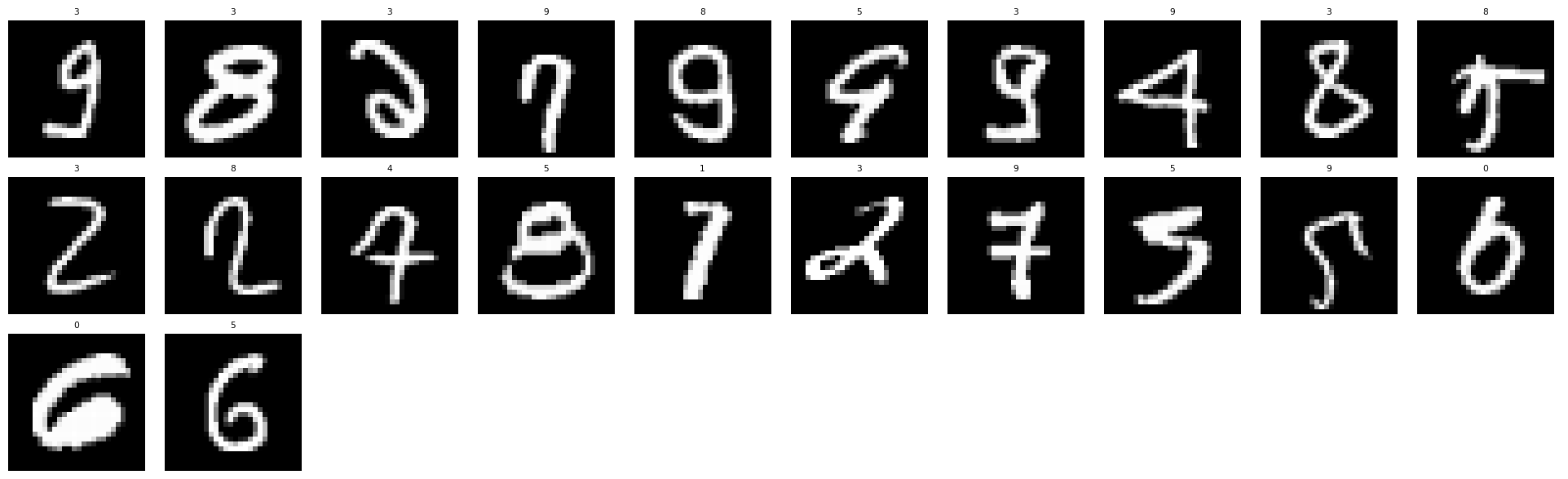
Looking at the misclassified examples reveals that many are genuinely ambiguous even to human readers. Some digits are written in unusual styles, have stray marks, or could reasonably be interpreted as multiple different digits. This is a common finding in classification tasks: the examples that remain difficult for the model after training are often the ones that would challenge human annotators as well.
Hyperparameter choices
The architecture and hyperparameters used above are not the result of exhaustive optimization. The number of filters (16 and 32), the filter size (3×3), the number of dense units (128), the learning rate (0.001), and the momentum (0.9) are all choices that could be tuned. In practice, these values often come from a combination of established conventions in the field and experimentation on the specific dataset. For MNIST, which is a relatively simple dataset by modern standards, many different configurations will work well. For more challenging tasks, careful hyperparameter tuning becomes increasingly important and can be the difference between a model that barely works and one that achieves state-of-the-art results.
14.4 Word Embeddings
The neural network architectures we have explored so far take numerical inputs: pixel intensities for images or measured quantities for tabular data. Text data presents a different challenge. Words are discrete symbols with no inherent numerical representation. The word “cat” is not naturally closer to “dog” than it is to “democracy” in any obvious numerical sense. Before we can apply neural networks to text, we need a way to represent words as vectors of numbers.
The simplest approach is called one-hot encoding. If our vocabulary contains \(V\) distinct words, we represent each word as a vector of length \(V\) with a single 1 in the position corresponding to that word and 0s everywhere else. For example, if our vocabulary is {“cat”, “dog”, “house”}, we might represent “cat” as \([1, 0, 0]\), “dog” as \([0, 1, 0]\), and “house” as \([0, 0, 1]\). This approach has two serious problems. First, the vectors are extremely long for realistic vocabularies (tens of thousands of words), making computation expensive. Second, all words are equally distant from all other words. The representation contains no information about semantic relationships.
Word embeddings solve both problems by learning dense, low-dimensional vectors that capture semantic meaning. Instead of a sparse vector with thousands of dimensions, each word is represented by a dense vector with perhaps 100 to 300 dimensions. More importantly, words with similar meanings end up with similar vectors. The word “cat” will be closer to “dog” than to “democracy” because both are animals that people keep as pets.
The key insight behind learning word embeddings is that words appearing in similar contexts tend to have similar meanings. This is known as the distributional hypothesis. If we see the sentences “The cat sat on the mat” and “The dog sat on the mat,” we learn something about the relationship between “cat” and “dog”: they can appear in the same contexts. Word embedding algorithms exploit this insight by training neural networks to predict words from their contexts (or vice versa), and the learned internal representations become the word vectors.
14.5 Movie Reviews Data
To illustrate word embeddings, we will work with a collection of movie reviews. Each review is a short text expressing an opinion about a film. We load the data and examine its structure.
imdb5k
shape: (5_000, 5)
| id | label | text | index | e5 |
|---|---|---|---|---|
| str | str | str | str | list[f64] |
| "doc0001" | "negative" | "In my opinion, this movie is n… | "test" | [-0.253192, 0.099743, … -0.000806] |
| "doc0002" | "positive" | "Loved today's show!!! It was a… | "test" | [0.280815, -0.064508, … -0.0273] |
| "doc0003" | "negative" | "Nothing about this movie is an… | "test" | [-0.179638, 0.171097, … 0.007573] |
| "doc0004" | "positive" | "Even though this was a disaste… | "train" | [0.300824, 0.027666, … -0.028764] |
| "doc0005" | "positive" | "I cannot believe I enjoyed thi… | "test" | [0.319154, 0.035425, … 0.001316] |
| … | … | … | … | … |
| "doc4996" | "positive" | ""Americans Next Top Model" is … | "test" | [0.305853, 0.026326, … 0.006194] |
| "doc4997" | "negative" | "It's very sad that Lucian Pint… | "train" | [0.217778, 0.283147, … -0.028361] |
| "doc4998" | "positive" | "Ruth Gordon at her best. This … | "train" | [0.373751, 0.076117, … -0.032517] |
| "doc4999" | "negative" | "I actually saw the movie befor… | "test" | [-0.073533, 0.10723, … 0.019535] |
| "doc5000" | "positive" | "I've Seen The Beginning Of The… | "test" | [0.147752, -0.095977, … -0.02008] |
Each row contains a review text and a sentiment label indicating whether the review is positive or negative. For learning embeddings, we focus on the text itself. The first step is to convert each review into a list of words, a process called tokenization. We use a simple approach that converts text to lowercase and splits on whitespace and punctuation.
imdb5k = (
    imdb5k
    .with_columns(
        tokens = c.text.str.to_lowercase().str.extract_all(r"[a-z]+")
    )
)
imdb5k
shape: (5_000, 6)
| id | label | text | index | e5 | tokens |
|---|---|---|---|---|---|
| str | str | str | str | list[f64] | list[str] |
| "doc0001" | "negative" | "In my opinion, this movie is n… | "test" | [-0.253192, 0.099743, … -0.000806] | ["in", "my", … "movie"] |
| "doc0002" | "positive" | "Loved today's show!!! It was a… | "test" | [0.280815, -0.064508, … -0.0273] | ["loved", "today", … "disappointed"] |
| "doc0003" | "negative" | "Nothing about this movie is an… | "test" | [-0.179638, 0.171097, … 0.007573] | ["nothing", "about", … "zero"] |
| "doc0004" | "positive" | "Even though this was a disaste… | "train" | [0.300824, 0.027666, … -0.028764] | ["even", "though", … "movie"] |
| "doc0005" | "positive" | "I cannot believe I enjoyed thi… | "test" | [0.319154, 0.035425, … 0.001316] | ["i", "cannot", … "an"] |
| … | … | … | … | … | … |
| "doc4996" | "positive" | ""Americans Next Top Model" is … | "test" | [0.305853, 0.026326, … 0.006194] | ["americans", "next", … "next"] |
| "doc4997" | "negative" | "It's very sad that Lucian Pint… | "train" | [0.217778, 0.283147, … -0.028361] | ["it", "s", … "of"] |
| "doc4998" | "positive" | "Ruth Gordon at her best. This … | "train" | [0.373751, 0.076117, … -0.032517] | ["ruth", "gordon", … "episode"] |
| "doc4999" | "negative" | "I actually saw the movie befor… | "test" | [-0.073533, 0.10723, … 0.019535] | ["i", "actually", … "money"] |
| "doc5000" | "positive" | "I've Seen The Beginning Of The… | "test" | [0.147752, -0.095977, … -0.02008] | ["i", "ve", … "film"] |
The tokenized text is now a list of words for each review.
14.6 Word2Vec
The most influential word embedding algorithm is Word2Vec, introduced by researchers at Google in 2013. Word2Vec comes in two variants: Skip-gram, which predicts context words given a target word, and CBOW (Continuous Bag of Words), which predicts a target word given its context. Both variants produce high-quality embeddings, but Skip-gram often works better for smaller datasets and rare words.
The Word2Vec model is itself a specific kind of neural network. We can represent the model in a digram format as shown in Figure Figure 14.5.
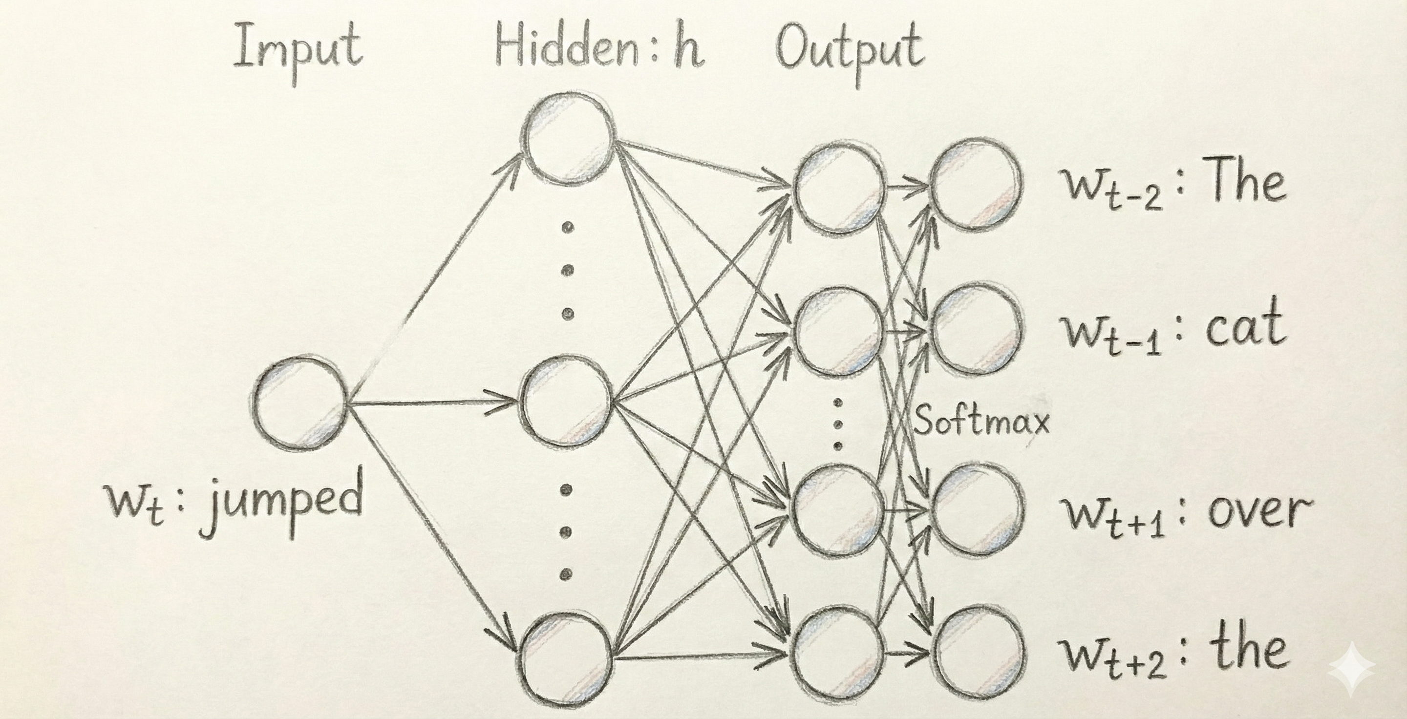
Training this model in PyTorch is certainly possible, but a bit complex because the embeddings on the left-side of the equation (the one that takes “jumped” as an input in the exam) need to be the same as the embeddings used to compare to the surrounding words on the right-side of the equation. Rather than implementing this logic ourselves, we use the gensim library to build Word2Vec embeddings using our movie reviews. The model takes several hyperparameters: vector_size controls the dimensionality of the embeddings, window specifies how many words on each side of the target word to consider as context, min_count filters out rare words that appear fewer than this many times, and sg=1 selects the Skip-gram variant.
model = Word2Vec(
    sentences=imdb5k["tokens"].to_list(),
    vector_size=100,
    window=2,
    min_count=5,
    sg=1,
    epochs=20
)
Exception ignored in: 'gensim.models.word2vec_inner.our_dot_float'
Exception ignored in: 'gensim.models.word2vec_inner.our_dot_float'
Exception ignored in: 'gensim.models.word2vec_inner.our_dot_float'
Exception ignored in: 'gensim.models.word2vec_inner.our_dot_float'
Exception ignored in: 'gensim.models.word2vec_inner.our_dot_float'
Exception ignored in: 'gensim.models.word2vec_inner.our_dot_float'
Exception ignored in: 'gensim.models.word2vec_inner.our_dot_float'
Exception ignored in: 'gensim.models.word2vec_inner.our_dot_float'
Exception ignored in: 'gensim.models.word2vec_inner.our_dot_float'The trained model contains a vocabulary of words and their corresponding embedding vectors. We can examine the size of the learned vocabulary and retrieve the embedding for any word.
len(model.wv)12479Each word is now represented as a vector of 100 numbers. We can convert this into a DataFrame using the following code:
embed = pl.DataFrame({
    "word": list(set(model.wv.key_to_index)),
    "embedding": [model.wv[w].tolist() for w in set(model.wv.key_to_index)],
})
embed
shape: (12_479, 2)
| word | embedding |
|---|---|
| str | list[f64] |
| "mitch" | [-0.15165, 0.409238, … -0.123146] |
| "binoche" | [0.067627, 0.321296, … 0.117199] |
| "become" | [-0.39514, 0.565347, … -0.867578] |
| "high" | [0.135096, -0.403576, … -0.048746] |
| "part" | [-0.017087, 0.55523, … -0.010798] |
| … | … |
| "jude" | [-0.42483, 0.124679, … -0.063253] |
| "bunker" | [0.024075, 0.201936, … -0.307226] |
| "carroll" | [-0.177406, 0.262557, … 0.130802] |
| "scheme" | [-0.326837, 0.476789, … 0.243038] |
| "refers" | [-0.570136, 0.317578, … -0.406813] |
As with the output from the dimensionality reduction algorithms in Chapter 12, the individual numbers have no intrinsic meaning. What matters are the relationships between the embeddings for different words.
14.7 Semantic Relationships
The power of word embeddings lies in their ability to capture semantic relationships. Words with similar meanings should have similar vectors, which we can measure using cosine similarity. The gensim model provides a convenient method to find the words most similar to a given word.
model.wv.most_similar("good", topn=10)[('decent', 0.6741176843643188),
('bad', 0.6352070569992065),
('great', 0.60764479637146),
('cool', 0.5773347020149231),
('ok', 0.558770477771759),
('lousy', 0.5540147423744202),
('promising', 0.5533482432365417),
('stellar', 0.5521603226661682),
('reasonable', 0.5515915751457214),
('goofy', 0.547494113445282)]The results show words that appear in similar contexts to “good” in our movie review corpus. Words like “great,” “bad,” and “excellent” appear because they are used in similar ways when expressing opinions about films.
We can also explore relationships for other types of individual words. Perhaps the most interesting thing, however, is looking at the relationships between multiple words all at once. The 100-dimensional embedding space is difficult to visualize directly. We can use the dimensionality reduction algorithms from Chapter 12 to reduce their dimenionality to make them possible to plot.
terms = pl.DataFrame({
    "word": ["good", "great", "excellent", "bad", "terrible", "awful",
             "movie", "film", "actor", "actress", "director",
             "love", "hate", "boring", "exciting", "funny", "scary"]
})

(
    terms
    .join(embed, on="word", how="inner")
    .pipe(
        DSSklearn.umap,
        features=[c.embedding],
        n_neighbors=4
    )
    .predict(full=True)
    .pipe(ggplot, aes("dr0", "dr1"))
    + geom_text(aes(label="word"))
    + theme_minimal()
)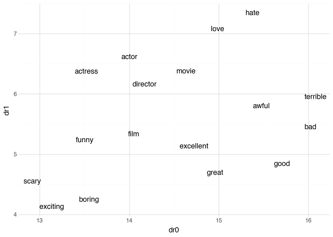
The visualization shows that semantically related words cluster together in the embedding space. Positive sentiment words like “good,” “great,” and “excellent” appear near each other, as do negative words like “bad,” “terrible,” and “awful.” Words related to film roles like “actor,” “actress,” and “director” form another cluster.
14.8 CNNs for Text
The word embeddings we learned in the previous section give us a way to represent individual words as dense vectors that capture semantic meaning. Now we turn to the question of how to use these representations for text classification. Given a movie review, can we predict whether it expresses a positive or negative sentiment?
One approach would be to use the averaged document vectors we computed at the end of the previous section as features for a traditional classifier. This works reasonably well but throws away information about word order. The sentence “not good” has a very different meaning from “good, not” but averaging the word vectors for both would produce similar results since they contain the same words. To capture patterns that depend on word order and local context, we turn to convolutional neural networks.
Recall that in image classification, a 2D convolutional layer slides a small filter across the image, computing a weighted sum at each position. The filter detects local patterns like edges or textures regardless of where they appear in the image. The same idea applies to text, but in one dimension rather than two.
When we represent a document as a sequence of word embeddings, we get a two-dimensional array: one dimension for position in the sequence (which word) and one for the embedding features (the 100 values representing each word). A 1D convolutional filter slides along the sequence dimension, looking at several consecutive words at a time. A filter of width 3 examines three adjacent word vectors and computes a weighted combination of all their features.
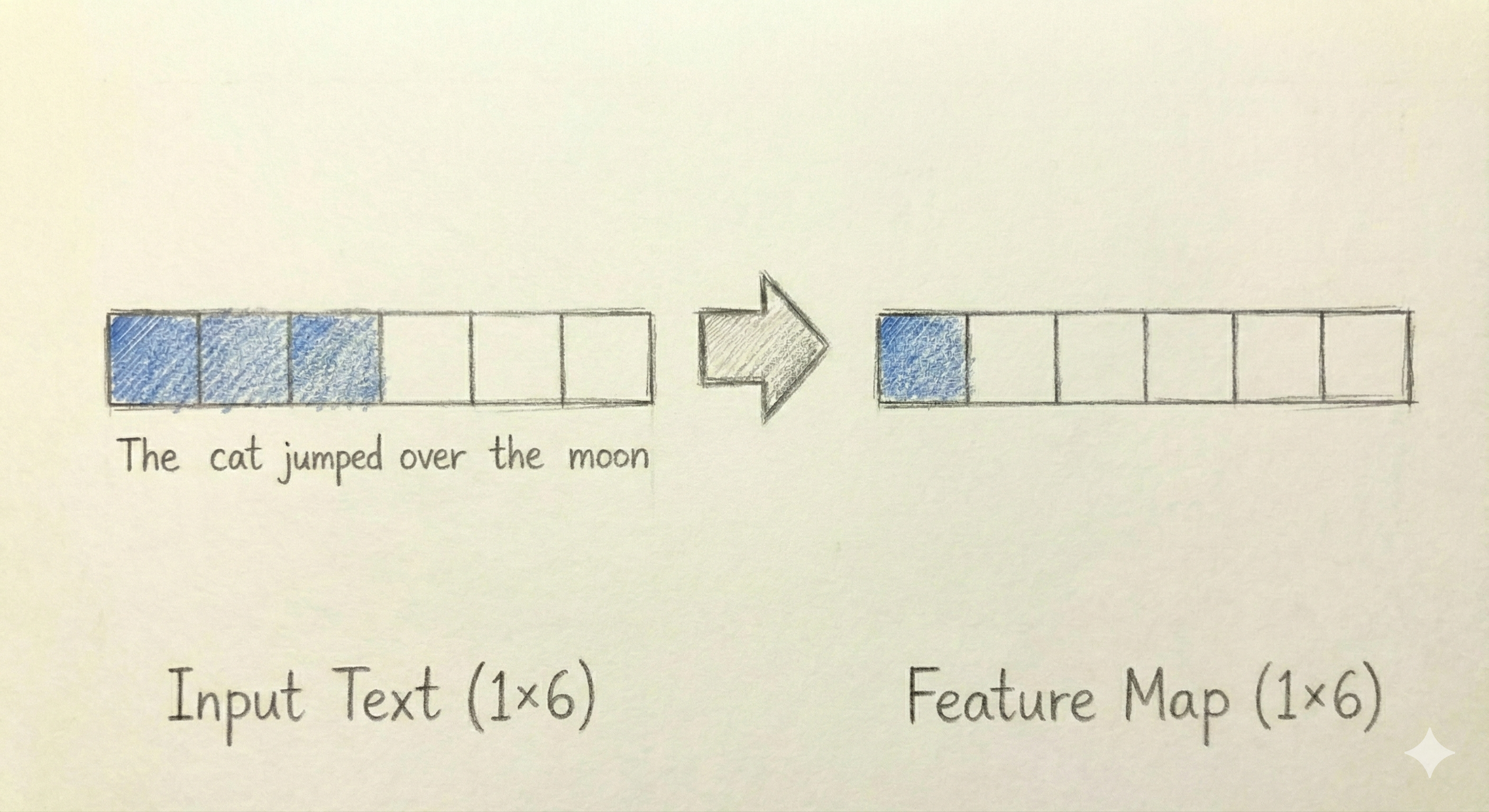
Consider what such a filter might learn. A filter could activate strongly when it sees the pattern “not good” or “not bad” — sequences where a negation word precedes a sentiment word. Another filter might detect emphatic phrases like “really great” or “absolutely terrible.” Each filter learns to recognize a different local pattern, and the collection of filters together captures many aspects of how sentiment is expressed in text.
After the convolutional layer processes the sequence, we have a new sequence of values — one output per filter for each position where the filter was applied. To produce a fixed-length representation regardless of document length, we apply global max pooling: for each filter, we take the maximum value it produced anywhere in the document. This captures whether a particular pattern appeared at all, regardless of where. The resulting vector has one value per filter and can be passed through dense layers to produce the final classification.
To build a text CNN in PyTorch, we need to prepare our data in a specific format. Each document must be converted to a sequence of integer indices that refer to positions in our vocabulary. We also need to handle the fact that documents have different lengths by padding shorter documents and truncating longer ones to a fixed maximum length. representing negative.
X, X_train, X_test, y, y_train, y_test, cn = DSTorch.load_text(
    df=imdb5k,
    model=model,
    tokens_expr=c.tokens,
    label_expr=c.label
)
A key component of our text CNN is the embedding layer, which converts word indices into embedding vectors. PyTorch provides nn.Embedding for this purpose. We can initialize this layer with the pre-trained Word2Vec embeddings we learned earlier, giving the model a head start with meaningful word representations.
embedding_dim = model.vector_size
embedding_matrix = torch.tensor(model.wv.vectors, dtype=torch.float32)
We now define the complete CNN architecture for text classification. The model consists of an embedding layer initialized with our Word2Vec vectors, a 1D convolutional layer that detects local patterns, global max pooling to aggregate across the sequence, and dense layers to produce the final classification.
class TextCNN(nn.Module):
    def __init__(self, embedding_matrix, num_filters=100, filter_size=3, num_classes=2):
        super().__init__()
        vocab_size, embedding_dim = embedding_matrix.shape

        self.embedding = nn.Embedding(vocab_size, embedding_dim)
        self.embedding.weight = nn.Parameter(embedding_matrix)
        self.embedding.weight.requires_grad = False

        self.conv = nn.Conv1d(
            in_channels=embedding_dim,
            out_channels=num_filters,
            kernel_size=filter_size,
            padding=filter_size // 2
        )
        self.relu = nn.ReLU()

        self.classifier = nn.Sequential(
            nn.Linear(num_filters, 64),
            nn.ReLU(),
            nn.Dropout(0.5),
            nn.Linear(64, num_classes)
        )

    def forward(self, x):
        embedded = self.embedding(x)
        embedded = embedded.permute(0, 2, 1)
        conv_out = self.relu(self.conv(embedded))
        pooled = conv_out.max(dim=2)[0]

        output = self.classifier(pooled)
        return output
The architecture deserves careful examination. The embedding layer converts each word index into its 100-dimensional vector. The permute operation rearranges the dimensions so that the embedding features become the “channels” that the 1D convolution operates over, and the sequence positions become the spatial dimension the filter slides along.
The convolutional layer nn.Conv1d applies num_filters different filters, each of width filter_size. With filter_size=3, each filter looks at three consecutive words. The padding ensures the output sequence has the same length as the input. After the ReLU activation, we take the maximum value across all positions for each filter using max(dim=2). This global max pooling produces a fixed-length vector regardless of input length.
The classifier head consists of two dense layers with dropout for regularization. Dropout randomly sets a fraction of the values to zero during training, which helps prevent overfitting by forcing the network to learn redundant representations.
Freezing embeddings
In the model above, we set requires_grad = False for the embedding weights. This freezes the pre-trained Word2Vec vectors, preventing them from being modified during training. This is appropriate when we have limited training data and want to preserve the semantic relationships learned from the larger corpus. With more training data, we could allow the embeddings to be fine-tuned by setting requires_grad = True, which might improve performance by adapting the representations to the specific task.
We create an instance of the model and set up the optimizer and loss function. For binary classification, we use cross-entropy loss, which is the standard choice for classification problems.
model_cnn = TextCNN(embedding_matrix, num_filters=100, filter_size=3)
optimizer = optim.Adam(model_cnn.parameters(), lr=0.001)
The training loop iterates over the training data in batches, computing predictions, calculating the loss, and updating the model parameters through backpropagation.
DSTorch.train(model_cnn, optimizer, X_train, y_train)Epoch 1/18, Loss: 0.6766
Epoch 2/18, Loss: 0.4758
Epoch 3/18, Loss: 0.3561
Epoch 4/18, Loss: 0.2467
Epoch 5/18, Loss: 0.1628
Epoch 6/18, Loss: 0.0870
Epoch 7/18, Loss: 0.0544
Epoch 8/18, Loss: 0.0308
Epoch 9/18, Loss: 0.0158
Epoch 10/18, Loss: 0.0099
Epoch 11/18, Loss: 0.0096
Epoch 12/18, Loss: 0.0060
Epoch 13/18, Loss: 0.0060
Epoch 14/18, Loss: 0.0040
Epoch 15/18, Loss: 0.0031
Epoch 16/18, Loss: 0.0033
Epoch 17/18, Loss: 0.0055
Epoch 18/18, Loss: 0.0039After training, we evaluate the model on both the training and test sets to assess how well it has learned and how well it generalizes to new examples.
DSTorch.score_text(model_cnn, X_train, y_train)1.0DSTorch.score_text(model_cnn, X_test, y_test)0.8349999785423279The model learns to classify sentiment from the movie reviews by detecting local patterns in the word sequences. The convolutional filters learn to recognize phrases and word combinations that are indicative of positive or negative sentiment.
14.9 Pre-trained embeddings
Training word embeddings on a small corpus like our movie reviews has limitations. Rare words may not have good representations, and the learned relationships reflect only the patterns in this specific dataset. In practice, it is common to use pre-trained embeddings learned from massive text corpora containing billions of words. Popular options include Word2Vec trained on Google News, GloVe trained on Wikipedia and web text, and fastText trained on Common Crawl. These pre-trained embeddings capture general semantic relationships and can be fine-tuned or used directly for downstream tasks. The gensim library provides tools for loading many pre-trained embedding models.
The gensim library includes a downloader that provides access to several pre-trained models. We can list the available models and load them directly.
import gensim.downloader as api

print(list(api.info()['models'].keys()))
['fasttext-wiki-news-subwords-300', 'conceptnet-numberbatch-17-06-300', 'word2vec-ruscorpora-300', 'word2vec-google-news-300', 'glove-wiki-gigaword-50', 'glove-wiki-gigaword-100', 'glove-wiki-gigaword-200', 'glove-wiki-gigaword-300', 'glove-twitter-25', 'glove-twitter-50', 'glove-twitter-100', 'glove-twitter-200', '__testing_word2vec-matrix-synopsis']The list includes models of varying sizes and training corpora. For our purposes, we will use glove-wiki-gigaword-100, which provides 100-dimensional GloVe embeddings trained on Wikipedia and Gigaword news text. This model strikes a balance between quality and computational efficiency.
pretrained = api.load("glove-wiki-gigaword-100")The loaded model works similarly to our Word2Vec model. We can query it for word vectors and find similar words. Let’s compare the most similar words to “good” in the pre-trained model versus our corpus-specific model.
pretrained.most_similar("good", topn=10)[('better', 0.893191397190094),
('sure', 0.8314563035964966),
('really', 0.8297762274742126),
('kind', 0.8288268446922302),
('very', 0.8260800242424011),
('we', 0.8234356045722961),
('way', 0.8215397596359253),
('think', 0.8205099105834961),
('thing', 0.8171301484107971),
("'re", 0.8141681551933289)]The results differ from our corpus-trained model because the pre-trained embeddings reflect patterns from general English text rather than movie reviews specifically. Notice that words related to quality and evaluation appear prominently. The pre-trained model has a much larger vocabulary, covering words that might appear rarely or not at all in our movie reviews.
len(pretrained)400000To use pre-trained embeddings with our text CNN, we need to create a new embedding matrix that maps our corpus vocabulary to the pre-trained vectors. Words that exist in the pre-trained model get their learned vectors; words that do not exist get random vectors initialized in the same range.
vocab = list(model.wv.key_to_index.keys())
embedding_dim = pretrained.vector_size

pretrained_matrix = np.zeros((len(vocab), embedding_dim))
found_count = 0

for i, word in enumerate(vocab):
    if word in pretrained:
        pretrained_matrix[i] = pretrained[word]
        found_count += 1
    else:
        pretrained_matrix[i] = np.random.uniform(-0.25, 0.25, embedding_dim)

print(f"Found {found_count} of {len(vocab)} words in pre-trained embeddings")
pretrained_matrix = torch.tensor(pretrained_matrix, dtype=torch.float32)
Found 12430 of 12479 words in pre-trained embeddingsMost words in our vocabulary have corresponding pre-trained vectors because they are common English words. The few missing words are typically misspellings, informal variants, or domain-specific terms.
We can now create a new text CNN using the pre-trained embedding matrix instead of our corpus-trained embeddings. The architecture remains identical; only the initial word vectors differ.
model_pretrained = TextCNN(pretrained_matrix, num_filters=100, filter_size=3)
optimizer_pretrained = optim.Adam(model_pretrained.parameters(), lr=0.001)
DSTorch.train(model_pretrained, optimizer_pretrained, X_train, y_train)Epoch 1/18, Loss: 0.6826
Epoch 2/18, Loss: 0.5154
Epoch 3/18, Loss: 0.3861
Epoch 4/18, Loss: 0.3002
Epoch 5/18, Loss: 0.2154
Epoch 6/18, Loss: 0.1435
Epoch 7/18, Loss: 0.0852
Epoch 8/18, Loss: 0.0567
Epoch 9/18, Loss: 0.0276
Epoch 10/18, Loss: 0.0184
Epoch 11/18, Loss: 0.0120
Epoch 12/18, Loss: 0.0057
Epoch 13/18, Loss: 0.0043
Epoch 14/18, Loss: 0.0034
Epoch 15/18, Loss: 0.0025
Epoch 16/18, Loss: 0.0028
Epoch 17/18, Loss: 0.0020
Epoch 18/18, Loss: 0.0020DSTorch.score_text(model_pretrained, X_train, y_train)
DSTorch.score_text(model_pretrained, X_test, y_test)0.8320000171661377The model with pre-trained embeddings often achieves comparable or better performance, particularly when the training corpus is small. The pre-trained embeddings provide a better starting point because they encode semantic relationships learned from billions of words of text.
14.10 Conclusion
This chapter introduced two powerful ideas that extend deep learning beyond the dense feedforward networks of Chapter 13. Convolutional neural networks exploit spatial structure in data by using local filters that detect patterns regardless of their position. For images, 2D convolutions slide across height and width to find edges, textures, and shapes. For text, 1D convolutions slide across sequences of words to find phrases and patterns that indicate meaning.
Word embeddings transform the discrete symbols of language into continuous vectors that capture semantic relationships. Words that appear in similar contexts end up with similar vectors, allowing neural networks to generalize across related words. Training embeddings on task-specific corpora produces representations tailored to the domain, while pre-trained embeddings from large general corpora provide a strong starting point that transfers well to many tasks.
The combination of word embeddings and convolutional networks creates a complete pipeline for text classification. The embedding layer converts words to vectors, convolutions detect local patterns like negation or emphasis, and pooling aggregates these detections into a fixed-length representation for classification. This approach captures information about word order that simpler bag-of-words methods discard.
The techniques in this chapter represent important steps in the development of modern deep learning, but they are not the final word. Recurrent neural networks process sequences one element at a time while maintaining memory of what came before, making them particularly suited to variable-length text. Transformer architectures use attention mechanisms to relate all positions in a sequence simultaneously, achieving remarkable performance on language tasks. Pre-trained language models like BERT and GPT extend the idea of pre-trained embeddings to entire contextual representations, where the same word gets different vectors depending on its surrounding context. These more recent approaches have largely superseded CNNs for text classification in research settings, though CNNs remain useful for their simplicity and efficiency. The foundations laid in this chapter, particularly the ideas of local pattern detection and learned representations, remain central to understanding these more advanced methods.